Introduction
An image has a huge number of pixels, and a classifier works best with a few good numbers. Feature extraction and dimensionality reduction turn the long pixel vector into a short feature vector before classification. Extracting discriminative and reliable features is always the key step for image recognition and computer vision. It is the middle stage of the computer vision system in Bayes Decision and Classifiers.
Main idea
Every method here makes features the same way: $\mathbf{f}=\boldsymbol{\Phi}^T\mathbf{x}$, where each column of $\boldsymbol{\Phi}$ is one direction and each feature is the coordinate of $\mathbf{x}$ along it. The methods only differ in how they learn $\boldsymbol{\Phi}$ from training data. PCA picks the directions where all the data spreads the most. LDA picks the directions where the classes are pulled apart the most. Both answers come out as eigenvectors.
Overview
The whole topic is one matrix multiplication:
What each part is:
- is the image written as one long column of pixel values
- is a direction in the -dimensional space, and is how far lies along it
- is learned from a training database
- PCA learns from all the samples without labels, and LDA learns it using the class labels
Step 1: computer vision reduces dimensions
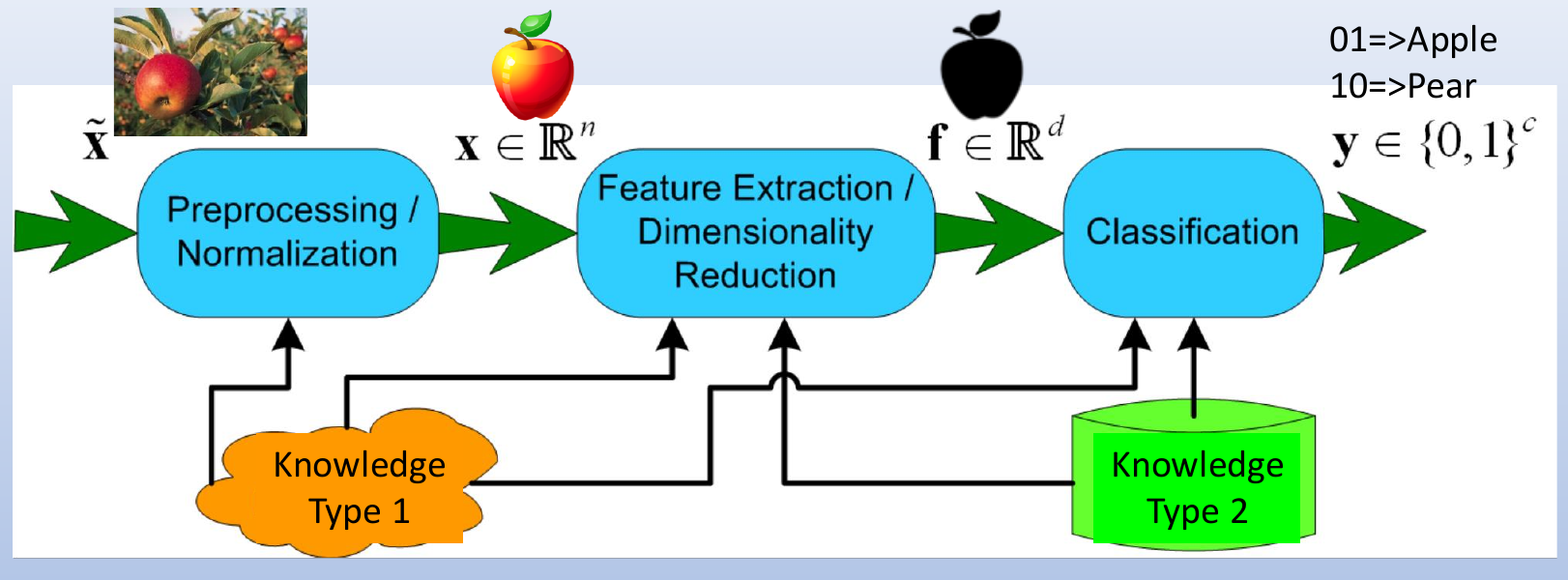
The two knowledge inputs in the figure are human knowledge and training samples. These notes learn the feature extraction from the training samples.
The sizes along the system are (the raw image), (the measured data after preprocessing, such as cropping or resizing), (the features, written with dimensions from here on) and (the class output, for example for apple and for pear), where often:
Reading the inequality from left to right, every stage throws away dimensions. So computer vision is a series of processes that:
- reduce the dimensionality of the samples
- reduce the variation of samples of the same class
- keep the discrimination between different classes
This gives two goals at the same time: dimensionality reduction and discriminative information extraction.
Step 2: where features come from
Feature extraction and dimensionality reduction can be based on:
- human expert knowledge
- image local structures
- image global structure
- machine learning and training data analysis
- deep learning, CNN and Transformer
The notes in this folder use machine learning and training data analysis.
Step 3: learning the transform from data
Take all pixels of the whole image as the initial features, and let the machine learn the effective features.
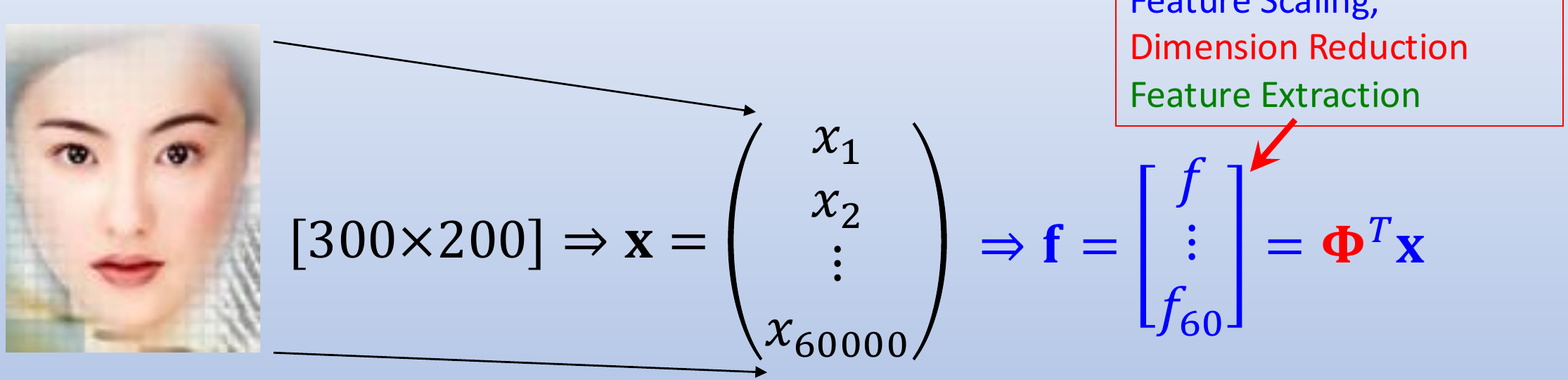
How it works, step by step:
- stack the pixels of a image into one vector
- multiply by a learned transform to get , so is
- each feature is a weighted sum of all pixels, so this single step weights (scales) the pixels, cuts numbers down to , and builds new features, all at once
- the transform is found by machine (computer) learning, also called training, from an image database such as a face database
Why fewer dimensions helps:
- a Gaussian classifier from the Bayes notes needs an covariance matrix per class, and since it is symmetric that is different numbers, far too many to estimate when is the number of pixels
- a database usually has far fewer images than pixels
- every later step costs less time and memory with numbers than with
Notation
These notes use different letters from the Bayes classifier notes:
| Meaning | Here | In the Bayes notes |
|---|---|---|
| number of dimensions of | ||
| number of training samples | ||
| number of samples in class | ||
| number of dimensions kept | ||
| number of classes |
Other symbols that change meaning:
- the feature vector is in this note and in all later notes (in the figure above, is the class output)
- the tilde in means the raw image in this note, and a centred sample in all later notes
- other sources may swap the letters, for example for the number of features and for the number of samples per class, so fix which letter is which before starting
Reading order
The notes follow one line of thought, each step using the one before:
- Principal Component Analysis: which single direction represents all the data best? (best point, projection, error, Lagrange, eigenvalue as variance)
- PCA Reconstruction: keep directions, rebuild the sample, and measure what is lost
- Eigen-Decomposition: write the covariance matrix with its eigenvectors, see why the new features are uncorrelated, and see what PCA keeps and loses
- Scatter Matrices: why PCA can fail for classification, and how the spread splits into within-class and between-class parts
- Linear Discriminant Analysis: which directions separate the classes best, and why cannot always be inverted
- LDA Variants: the ways around a singular , and a summary of PCA and LDA
Concept map
flowchart TD
    A["f = Φᵀx<br/>learn the directions Φ"] --> B["PCA<br/>min reconstruction error ⇔ max φᵀSᵗφ<br/>Sᵗφ = λφ"]
    B --> C["PCA reconstruction<br/>error = sum of dropped λ<br/>rank Sᵗ ≤ q − 1"]
    C --> D["Eigen-decomposition<br/>Σ = ΦΛΦᵀ, features uncorrelated<br/>PCA: max trace(ΦᵀSᵗΦ)"]
    D --> E["Scatter matrices<br/>Sᵗ = Sʷ + Sᵇ"]
    E --> F["LDA<br/>max trace(Φᵀ(Sʷ)⁻¹SᵇΦ)"]
    F -->|"Sʷ singular"| G["LDA variants"]
Why do we need this
The Bayes classifiers need a covariance matrix and enough samples to estimate it. With raw pixels, neither is practical. These methods learn a short feature vector first, so the classifier has a small, well-estimated problem to solve.
Key math ideas
The math ideas this topic relies on, and where each one appears:
- Dot product and projection: each feature is a coordinate along one direction, in Principal Component Analysis, PCA Reconstruction and Projection onto an Axis
- Covariance matrix: , and are covariance matrices of different sets of points, in Scatter Matrices, Principal Component Analysis and Eigen-Decomposition
- Eigenvectors and eigenvalues: the PCA and LDA directions are eigenvectors, and the eigenvalues are the spread along them, in Principal Component Analysis, PCA Reconstruction, Eigen-Decomposition, Linear Discriminant Analysis and LDA Variants
- Lagrange multiplier: why the best direction of length 1 is an eigenvector, in Principal Component Analysis, Eigen-Decomposition and Linear Discriminant Analysis
- Gradient: setting the derivative to zero finds the mean and the best directions, in Principal Component Analysis and Linear Discriminant Analysis
- Inverse covariance and whitening: LDA needs , and the LDA Variants exist because it can fail to exist, in Linear Discriminant Analysis and LDA Variants
- Trace: the total, within-class and between-class spread, and the spread kept by a set of directions, in Scatter Matrices, Eigen-Decomposition, PCA Reconstruction and Linear Discriminant Analysis
- Rank: why the subspaces have sizes , and , in PCA Reconstruction, Linear Discriminant Analysis and LDA Variants
Visual 1: how the methods fit together
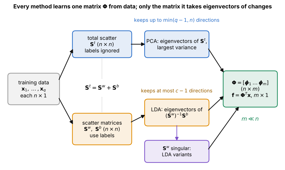
Read it from left to right:
- every method starts from the same training samples and ends with one matrix , so the features are always
- the top path ignores labels: PCA takes the eigenvectors of with the largest eigenvalues
- the bottom path uses labels: LDA takes the eigenvectors of , and the LDA variants step in when cannot be inverted, also ending with a
- links the two paths, and the reading order follows the top path first, then the bottom one