Introduction
Linear discriminant analysis (LDA) finds the projection directions that best separate the classes. It uses the class labels through the scatter matrices, so it is a supervised method. It keeps the directions with the most between-class spread for each unit of within-class spread, which is what classification needs.
Main idea
LDA wants a small $\operatorname{trace}[\boldsymbol{\Phi}^T\mathbf{S}^w\boldsymbol{\Phi}]$ and a large $\operatorname{trace}[\boldsymbol{\Phi}^T\mathbf{S}^b\boldsymbol{\Phi}]$, combined as $\max\operatorname{trace}[\boldsymbol{\Phi}^T(\mathbf{S}^w)^{-1}\mathbf{S}^b\boldsymbol{\Phi}]=\sum_{k=1}^{m}\lambda_k^{b/w}$. The columns of $\boldsymbol{\Phi}$ are eigenvectors of $(\mathbf{S}^w)^{-1}\mathbf{S}^b$, and each eigenvalue is the ratio of between-class to within-class spread along its eigenvector. LDA needs $(\mathbf{S}^w)^{-1}$, which does not exist when $q-c
Overview
LDA is PCA with a different matrix inside the trace:
In both, is and the features are . Subtracting moves every sample by the same amount, so it does not change which directions separate the classes. Only the matrix whose eigenvectors are taken changes, from to .
Step 1: two goals
Scatter Matrices gave the two desired properties of a projection for classification. With directions in , written as traces:
What each trace is:
- diagonal entry of is , the within-class spread along direction , so the trace is the total within-class spread kept
- in the same way, is the total between-class spread kept
- one should be small and the other large at the same time
Step 2: combine into one ratio
For one direction , "top large and bottom small" is the same as "the ratio large". This is the Fisher ratio:
Why a ratio works:
- a large top means the projected class means are far apart
- a small bottom means each projected class is tight
- scaling by any number changes the top and bottom by the same factor, so only the direction matters and no length constraint is needed
Step 3: solve for the best direction
Set the gradient of to zero. Write and , and use the gradient rule from Principal Component Analysis with the quotient rule:
If can be inverted, multiply both sides on the left by :
What this says:
- the best direction is an eigenvector of , the same kind of answer as PCA with a different matrix
- its eigenvalue is the Fisher ratio it achieves, so the best direction has the largest eigenvalue
- is the matrix version of "between divided by within", which is where the inverse in the criterion comes from
A picture of what does:
- first whiten with : stretch and squash the space so that the within-class cloud becomes round with unit spread
- in that space the within-class spread is the same in every direction, so the best direction is simply where the class means spread the most, which is PCA on the class means
- turned back to the original space, these directions are the LDA directions, which is why they are perpendicular in the whitened space but not in general in the original one
Step 4: LDA criterion
Take the eigenvectors of the largest eigenvalues as the columns of . Diagonal entry of is then , so:
where are the eigenvalues of . Compare with PCA, which takes the eigenvalues of alone, and mixes the helpful and the unhelpful spread.
How to read this criterion with directions:
- this trace form is a shorthand: it is reached by the eigenvectors, and its value there is , the sum of the Fisher ratios of the chosen directions
- taken literally it has no length limit, so a more exact criterion is , which, like , does not change when is scaled and has the same eigenvectors as its answer
- taking the largest eigenvalues keeps the directions with the best class separation
- is the matrix version of "between divided by within", and the trace is not the same as divided by
One difference from PCA:
- is not symmetric, even though and are, so its eigenvectors are in general not orthogonal and
- the diagonal entry equals only when each eigenvector is taken with unit length
Step 5: how many features
is built from the vectors , and their weighted sum is zero: . So they span at most directions, by the same argument as the rank of in PCA Reconstruction:
A product of matrices has rank at most the rank of each factor, so has rank at most and at most nonzero eigenvalues, and LDA gives at most useful features. Two classes give one LDA feature.
Step 6: why LDA is preferred
Pattern recognition does not need to represent the original data. It needs to discriminate the class membership of the data. So:
- LDA extracts much more discriminative features than PCA
- the vast majority of researchers prefer LDA to PCA for feature extraction and dimensionality reduction for pattern recognition
Step 7: singular within-class scatter
LDA needs , and it often does not exist.
Why the rank of is at most :
- class has samples, and their offsets from add up to zero, so they span at most directions
- adds up the class covariances, so it spans at most directions
- it is , so its rank is also at most
What goes wrong:
- in many applications , for example a few hundred face images of tens of thousands of pixels each
- then has many zero eigenvalues, so its determinant, which is the product of its eigenvalues, is zero, it is singular, and its inverse does not exist
- along a direction with zero within-class spread, the bottom of is zero, so is infinite and the criterion has no finite best answer
- thousands of research papers proposed various LDA variants to solve this problem
Why this is more than a missing inverse:
- the zero within-class spread is measured on the training samples only
- class has training samples, so they spread in at most directions, and in every other direction they show no spread at all, even though new samples of the same class will spread there
- so with few samples, cannot be inverted, and it also misreports the true within-class spread
- the variants differ on what to do with these directions: some drop them, and some (NDA) treat them as the most discriminative
Why do we need this
It gives features chosen for the job of classification, using the labels. It is the same eigenvector machinery as PCA, applied to the ratio of between-class to within-class spread.
Next step
LDA Variants are the ways to make LDA work when cannot be inverted.
Visual 1: Fisher ratio as the direction turns
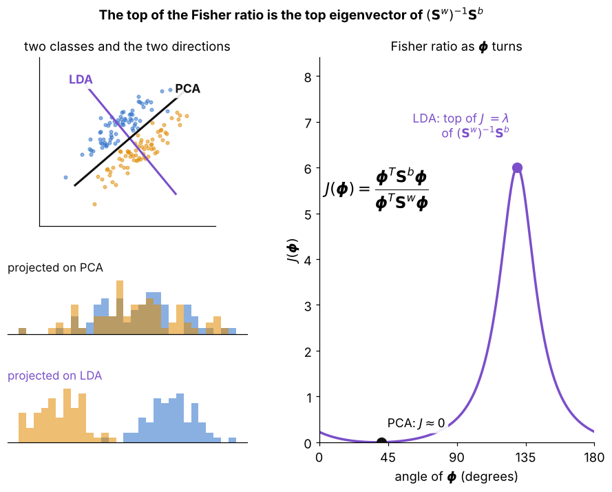
Two classes that are long and thin and lie side by side:
- right: worked out for every angle has one sharp peak, and its height is the largest eigenvalue of at that eigenvector, as Step 3 says
- left, top: the PCA direction lies along the long side of both classes, and the LDA direction cuts across them
- left, below: projected on PCA the two classes land on top of each other (), projected on LDA they come apart
- two classes give one useful LDA direction, as Step 5 says
Visual 2: whitening view of LDA
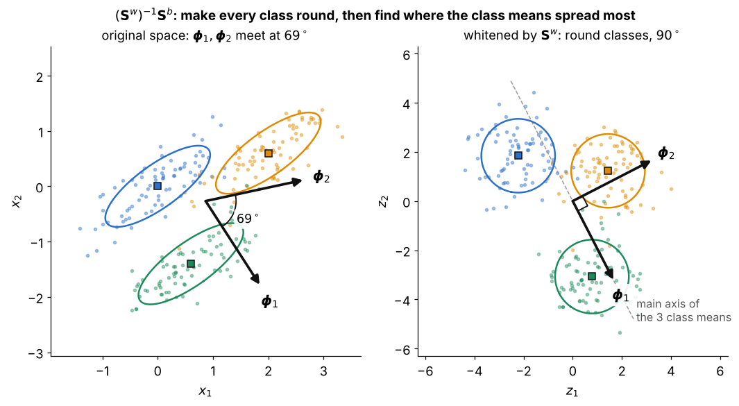
Three classes with the same tilted within-class shape, and the two LDA directions , ():
- left, original space: the LDA directions meet at , so they are not orthogonal, as Step 4 says
- right, after whitening with : every class becomes a round cloud with unit spread
- there the same two directions meet at a right angle, and lies along the main axis of the three class means (dashed), so LDA is PCA of the means
- this is the picture in Step 3: whiten, do PCA on the means, then map the directions back