Introduction
The rank of a matrix is the number of independent directions its outputs can point in (the general idea is in Rank and Nullity). For a covariance or scatter matrix built from samples, the rank is the number of directions in which the samples actually spread. The numbers , and keep appearing in Part 2 because of this, and they explain why some matrices cannot be inverted.
Main idea
A scatter matrix built from $q$ centred samples has rank at most $q-1$, because the offsets from the mean add up to zero. Splitting into $c$ classes removes one direction per class, so $\mathbf{S}^w$ has rank at most $q-c$, and the $c$ class means give $\mathbf{S}^b$ rank at most $c-1$. When the rank is below $n$, the matrix has zero eigenvalues, the data never moves in those directions, and the matrix has no inverse.
What it is
Three equal ways to say it, for a symmetric matrix such as a covariance:
- the number of independent columns
- the number of independent directions that its outputs can point in
- the number of nonzero eigenvalues
Physical meaning for data
Why a scatter matrix cannot have more directions than its samples give:
- is always a weighted sum of the centred samples
- so its outputs can only point in directions that the samples span
- the rank is the number of directions in which the data actually spreads
Where the minus ones come from:
- for : the offsets from the overall mean add up to zero, so the last one is fixed by the others
- for : inside each class the offsets from the class mean add up to zero, which removes one direction per class
- for : the weighted offsets of the class means from the overall mean add up to zero
What a rank below means:
- the matrix has zero eigenvalues, one per missing direction
- along those directions the training data shows no spread at all
- the matrix is singular, so its inverse does not exist and you cannot "divide by the spread" there
- with fewer samples than dimensions, which is normal for images, most directions of the space have no training data in them
Where it is used
| Note, step | What the rank tells you there |
|---|---|
| PCA Reconstruction, Step 4 | , so PCA features rebuild the training data with zero error |
| Linear Discriminant Analysis, Step 5 | , so LDA gives at most useful features |
| Linear Discriminant Analysis, Step 7 | , so with it is singular and plain LDA fails |
| LDA Variants | the variants work in subspaces sized , and , chosen so their matrices can be inverted |
| Discriminant Function in Eigenspace, Step 6 | a class covariance from samples has rank at most , so most of its eigenvalues are zero |
| Least Squares Single Layer Network, Step 3 | there is not centred, so its rank is at most ; with fewer samples than inputs it is singular and many weight vectors give the same smallest error |
| CNN as a Regularized MLP, Step 5 | weight sharing gives each weight many more examples, which is the network answer to having few samples in many dimensions |
Common traps
Points that are easy to get wrong:
- the rank limits are upper bounds; the rank can be lower if samples happen to line up
- a matrix with full rank can still be nearly singular: tiny eigenvalues are as harmful as zero ones for a classifier that divides by them
Test yourself
Why do two samples always lie on one line, even in a space of thousands of dimensions?
Their offsets from their mean are equal and opposite, so they point along one direction. The scatter matrix of two samples has rank at most 1.
Why can LDA give at most features?
The between-class scatter is built from class means whose weighted offsets add up to zero, so it covers at most directions. The product cannot have a higher rank than .
Why does PCA before LDA reduce to dimensions?
has rank at most , so it is singular in any larger space. In at most dimensions it has a chance to have no zero eigenvalues and be inverted.
Why do we need this
Rank is the reason the small-sample problem exists at all. It tells you how many directions the training data really fills, which features a method can give, and when a matrix the method needs cannot be inverted.
Visual 1: few samples fill few directions
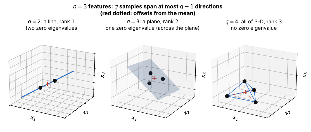
Each panel has features and random samples:
- : the offsets from the mean (red dotted) point along one line, so the scatter matrix has rank 1 and two zero eigenvalues
- : the samples lie in one plane, rank 2, and the eigenvalue across the plane is
- : four samples finally fill 3-D space, rank 3, with no zero eigenvalue
- in every panel the rank is , because the offsets from the mean add up to zero
Visual 2: rank of the scatter matrices as samples grow
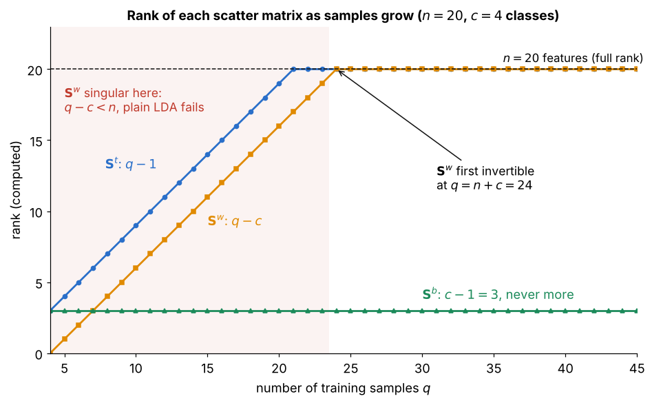
Ranks computed from random data with features and classes:
- grows as and as , until they reach the full
- stays at however many samples you add, which is why LDA gives at most features
- in the shaded part is singular, so does not exist and plain LDA fails
- first reaches full rank at ; with images, is so large that this is almost never reached