Introduction
This note applies maximum likelihood estimation to samples from a multivariate Gaussian with an unknown mean and an unknown covariance matrix . It works the 1-D case in full, then states the multivariate result. The ML estimates are the sample mean and the sample covariance, both with the factor .
Main idea
Take the log of the Gaussian, differentiate with respect to each parameter, add over the samples, and set to zero. The answers are $\hat{\boldsymbol{\mu}}=\frac{1}{n}\sum_{k=1}^{n}\mathbf{x}_k$ and $\hat{\boldsymbol{\Sigma}}=\frac{1}{n}\sum_{k=1}^{n}(\mathbf{x}_k-\hat{\boldsymbol{\mu}})(\mathbf{x}_k-\hat{\boldsymbol{\mu}})^T$: the average sample, and the average outer product of the deviations from it.
Overview
The parameters and their estimates, with of dimensions:
Step 1: log-likelihood of one sample
The multivariate Gaussian, the bell curve over features (Gaussian Discriminant Function explains it). is the mean vector, is the covariance matrix, with the variance of each feature on the diagonal and the covariance of each pair of features off the diagonal, is its determinant and its inverse:
Take of one sample :
Explaining each term:
- the front factor is , and , which gives the first term
- of the exponential is just its exponent, which gives the second term
- the first term depends only on , and the second is a distance of from scaled by
Step 2: univariate case
Consider first one dimension, , with two parameters :
In 1-D, becomes and becomes , so the log-likelihood of one sample simplifies to:
Step 3: gradient of one sample
Differentiate with respect to and with respect to , treating as one variable :
Where each entry comes from:
- top, : the first term has no , and for the second the chain rule gives , where is the derivative of with respect to
- bottom, with : , and , with
Step 4: apply ML and solve
Apply ML, . This gives one equation per parameter:
Solving the two equations:
- multiply the first by : , so
- multiply the second by : , so
- both equations hold at the same point, so the inside the second is the estimate from the first
So the maximum likelihood estimates are:
Step 5: multivariate result
The multivariate case follows the same steps with more manipulations. For the mean, the gradient of the second term of Step 1 with respect to is , the 1-D with replaced by . ML gives . Multiplying both sides by leaves , the vector version of the first equation in Step 4. For the covariance, the gradient is taken entry by entry of ; the steps are longer, and only the result is needed. The ML estimates for the mean vector and the covariance matrix of a multivariate Gaussian are:
How to read them:
- averages each feature over the samples, so it is the 1-D done for every feature at once
- each is a outer product, and its entry is the deviation of feature times the deviation of feature
- so a diagonal entry of is the 1-D of one feature, and an off-diagonal entry is the covariance of two features
Factor or
The ML estimate divides by . Dividing by instead gives the unbiased estimate of the covariance: averaged over many training sets it equals the true , while the version comes out a little too small, because is fitted to the same samples. The two are almost the same when is large.
With only a few samples per class, the ratio between the two is large, so use , the ML estimate, and say which one you used.
Why do we need this
These are the numbers a Gaussian classifier plugs in: estimate and from the samples of each class, and the Gaussian discriminant functions are ready to use.
Next step
The same sample covariance, computed over all samples together, is the starting point of Visual Data Dimensionality Reduction.
Visual 1: fitted ellipse against sample size
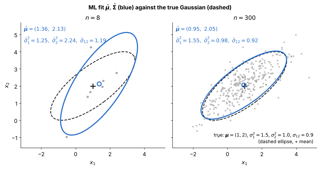
Each ellipse is the 2-standard-deviation contour of a Gaussian; dashed is the true one, blue is the ML fit:
- left, : and come from only eight points, so the fitted ellipse has the wrong size and tilt
- right, : the averages settle down, and the blue ellipse almost covers the dashed one
- and are the diagonal of and the off-diagonal, which sets the tilt
- this is why a Gaussian classifier needs many more samples per class than features
Visual 2: why is a little too small
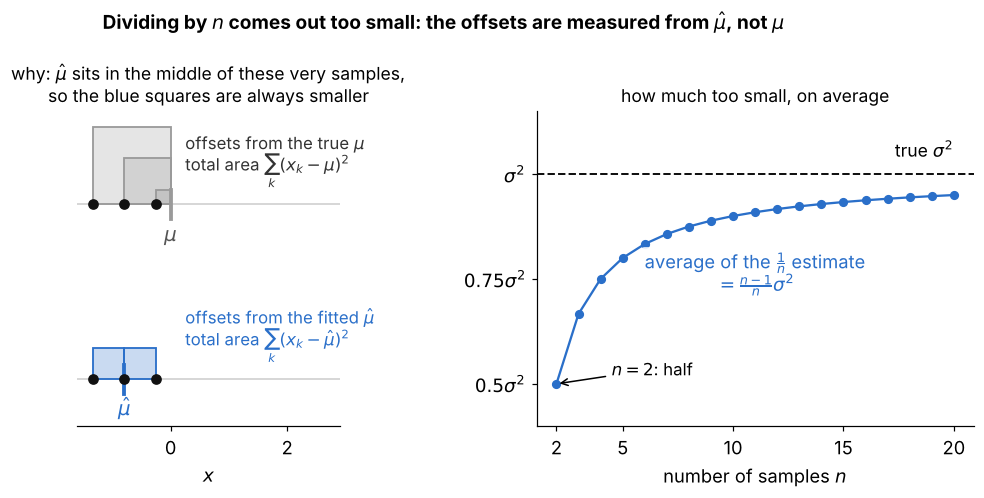
Left, one random set of 3 samples from a class with true mean ; each square has side , so its area is the squared offset:
- grey squares measure from the true , and blue squares measure from the fitted
- is the point that makes the total squared offset smallest for these very samples, so the blue total is never larger than the grey one
- the variance needs offsets from the true , so dividing the smaller blue total by comes out too small on average
- right: on average the estimate is , half the truth at and close to it for large , as the callout on against says