Introduction
Principal component analysis (PCA) asks: if each sample may keep fewer numbers, which directions should those numbers measure? It answers by making the reconstruction error as small as possible. It uses no class labels, so it is an unsupervised method. The answer is the eigenvectors of the covariance matrix of all the data, called the total scatter matrix .
Main idea
Replace each centred sample $\tilde{\mathbf{x}}_i$ by its shadow $a_i\boldsymbol{\phi}$ on a line through the mean, where $a_i=\boldsymbol{\phi}^T\tilde{\mathbf{x}}_i$. The error is $\varepsilon^2=\sum_i\|\tilde{\mathbf{x}}_i\|^2-q\,\boldsymbol{\phi}^T\mathbf{S}^t\boldsymbol{\phi}$, and the first term is fixed. So the smallest error comes from the largest $\boldsymbol{\phi}^T\mathbf{S}^t\boldsymbol{\phi}$ with $\boldsymbol{\phi}^T\boldsymbol{\phi}=1$, which gives $\mathbf{S}^t\boldsymbol{\phi}=\lambda\boldsymbol{\phi}$. The eigenvalue $\lambda$ is the variance along $\boldsymbol{\phi}$, so take the eigenvector with the largest eigenvalue.
Overview
The derivation is one chain. Each step below explains one link:
Setup
There are training samples of dimensions:
Each sample is a column vector (), so it is one point in an -dimensional space.
Step 1: best single point
Start with the extreme case: use one point to stand for all training samples. The best point makes the total squared distance to all samples smallest:
How to solve it:
- the gradient with respect to a vector is the vector of partial derivatives, one per component, and it is zero at a minimum
- each term is a squared length, , and its partial derivative with respect to component is , so its gradient is , just as
- set the total gradient to zero:
- this is , so:
The best single point is the sample mean. So every later description of the samples is measured from the mean. Just for simpler symbols, centralize the samples and put them side by side as the columns of an training data matrix:
After centring, the mean sits at the origin.
Step 2: project onto one direction
Now allow each sample to keep one number. Choose a direction given by a unit vector :
Project each centred sample onto it. The -dimensional is reduced to the one-dimensional number:
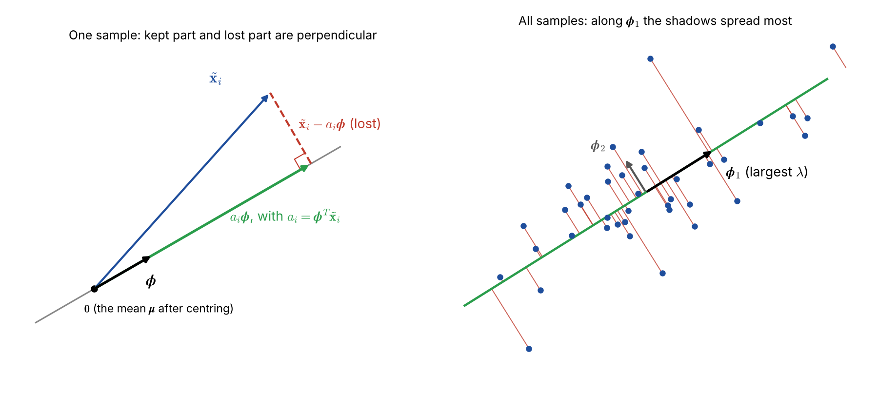
What each piece means (left panel):
- is the coordinate of along the line, like reading a ruler laid along , and since it equals , where is the angle between and
- is the point on the line where lands
- is the part that is lost
Why the lost part is perpendicular to the line, using :
Why is the best point on the line: any other point is further away, because is a sum of two perpendicular parts, so by Pythagoras:
So is the best rebuild of from one number.
The best direction makes the total lost part, the reconstruction error, smallest:
Step 3: expand the error
Write the squared length as a vector times its own transpose, and multiply out the brackets:
Simplify each term:
- , by the definition of
- is a single number, and a number equals its own transpose, so and the third term is also
- , because
So . Add over all samples:
Now write with outside. Since and also :
is the same for every sample, so it moves outside the sum:
What this says:
- the first term is the total spread of the data about its mean, and it does not depend on
- the second term is the spread that the line keeps
- geometrically this is Pythagoras on the right-angled triangle in the figure:
- so losing the least is the same as keeping the most
Step 4: total scatter matrix
The middle of the second term is times the sample covariance matrix of all the training data:
Why each form is the same:
- each is () times (), so it is an matrix
- is () times (), and multiplying column by row it equals
- it is called the total scatter matrix , because it uses all samples together, whatever their class
and are two names for the same matrix, and these notes use from here on.
What each entry is:
- entry of is , where is feature of sample
- a diagonal entry () is the variance of feature , how much it spreads
- an off-diagonal entry is the covariance of features and : positive if they tend to go up together, negative if one goes up when the other goes down, and zero if they are uncorrelated
- swapping and gives the same number, so is symmetric,
- the sum of the diagonal, the trace, is the total variance of all features
Substitute into Step 3:
So minimizing is maximizing , with the constraint .
Why the constraint is needed: without it, doubling multiplies by 4, so the maximum would be an infinitely long . We want a direction, so the length is fixed at 1.
Step 5: Lagrange optimization
A Lagrange multiplier puts the constraint into the function. Maximize:
Take the gradient with respect to , using two rules for a symmetric matrix :
- , because appears twice and each copy gives one term, and for a symmetric such as this is , the vector form of
- , which is the first rule with
The gradient with respect to gives back . So the solution is an eigenvalue and unit eigenvector of : a direction that only stretches by and does not turn.
Why this finds the best direction under the constraint, as a picture:
- must keep length 1, so it can only move around the sphere of unit vectors, which means it can only move sideways (perpendicular to itself)
- the score rises fastest along its gradient
- if has any sideways part, turning a little that way raises the score, so was not the best
- at the best , has no sideways part, so it points along , which is exactly
- the term is the algebra for this picture: its gradient points straight out of the sphere and removes the part of the gradient that would only change the length
Step 6: eigenvalue is the variance
is a symmetric matrix, so it has eigenvectors, and all of them satisfy Step 5, the worst one too. Step 5 only narrows the answer down to these candidates. To choose, look at what means.
Variance along any direction. Put the definition of in. Each term is the number times its own transpose:
The projected numbers have zero mean, because . So is their variance. This also explains why is the right quantity: the raw projections have mean , so is each projection minus the projected mean, which is exactly what the definition of variance squares and averages. It is the kept spread of Step 3, divided by . In words: for any covariance matrix and any unit vector, is the variance of the data projected onto .
Eigenvalue is the variance. For an eigenvector, multiply on the left by :
What follows:
- the eigenvalue of a covariance matrix is the variance of the data projected onto its eigenvector
- Step 5 says the best must be one of the eigenvectors, and at eigenvector the value of is , so the best one is the eigenvector with the largest eigenvalue, where is maximum and the reconstruction error is minimum
- this direction is the first principal component: the variance of the projected data is largest along it ( in the right panel of the figure, where is the other eigenvector, perpendicular to it, with the smaller eigenvalue)
- the eigenvector with the smallest eigenvalue is the worst direction, the one that loses the most
Summary
Read the chain from left to right:
- the best single point is the mean, so the samples are centred first
- keeping one number per sample means projecting onto a unit vector
- by Pythagoras, the smallest error is the largest kept spread
- with , Lagrange gives
- the eigenvalue is the kept variance, so take the eigenvector of the largest eigenvalue
Why do we need this
PCA gives the best description of the data in fewer dimensions, in the sense of the smallest squared reconstruction error. It needs only samples, no labels, and the answer is a standard eigenvector problem.
Next step
PCA Reconstruction keeps directions instead of one, and shows that the error is exactly the sum of the dropped eigenvalues.
Visual 1: kept and lost as the line turns
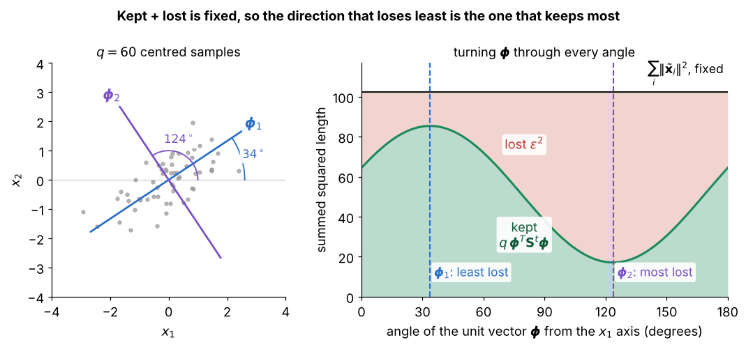
Left, the centred samples with and and their angles; right, the unit vector turned through every angle:
- green is the kept spread , and red is the lost part
- the black line does not move, so every gain in green is the same loss in red, which is the equation of Step 4
- the least loss is at the angle of , along the long side of the cloud, and the most loss at , across it, which is Step 6
Visual 2: best single point is the mean
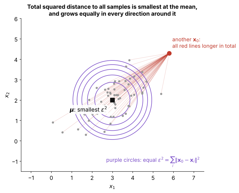
Step 1 as a picture: try every point and add up its squared distances to all samples:
- the red lines from one other point to every sample have a larger total squared length than lines from the mean would
- the purple circles join points with the same total , and they are all centred on
- the circles are round because : moving away from costs the same in every direction
- so the best single point is the mean, and every later description of the data is measured from it