Introduction
Many formulas in Part 2 multiply by an inverse: in the Gaussian classifier, in LDA, in least squares. They all do one physical thing: whitening, which squashes and stretches space until the data cloud is round. Once that picture is in place, the Mahalanobis distance, the tilt of the linear boundary, LDA and the small-eigenvalue problem become one idea (the distance itself is in Mahalanobis Distance in Pattern Recognition).
Main idea
$\boldsymbol{\Sigma}^{-1}$ has the same axes as $\boldsymbol{\Sigma}$ with spreads $\frac{1}{\lambda_k}$, so it shrinks the long axes and stretches the short ones. Whitening, $\mathbf{y}=\boldsymbol{\Lambda}^{-1/2}\boldsymbol{\Phi}^T(\mathbf{x}-\boldsymbol{\mu})$, turns onto the axes and divides each coordinate by its spread $\sqrt{\lambda_k}$, so the cloud becomes a round ball with unit spread. Every "divide by the spread" in Part 2 is this, and it is also where tiny eigenvalues do harm: dividing by a tiny spread blows up whatever lies along that axis.
What it is
What the inverse looks like in the eigenvector axes:
- , and
- same axes, reciprocal spreads
- it exists only if no is zero
The whitening transform:
- turns the cloud onto its own axes
- divides the coordinate along axis by , the spread along it
Physical meaning
What whitening does to the cloud:
- a long axis (large ) is squeezed, a short axis (small ) is stretched, until every axis has spread 1
- the tilted ellipse becomes a round ball, so after whitening no direction is special
- distances measured after whitening are in units of the cloud's own spread
What it explains:
- Mahalanobis distance is the ordinary squared distance after whitening:
- Gaussian classifiers are "whiten, then measure distance to the mean": with a shared every class is whitened the same way, so the boundary is the perpendicular bisector in the round space, which looks tilted in the original space (linear classifier); with the classes are already round (minimum distance classifier)
- LDA is "whiten with , then find where the class means spread most": after whitening every class is round, so only the spread of the means matters
- the small-eigenvalue problem: dividing by for a tiny, underestimated stretches that axis hugely, so any offset along it, including noise, looks enormous
- the fixes: adding caps how much any axis can be stretched, replacing small by a constant does the same, and PCA drops those axes before whitening
Where it is used
| Note, step | What the inverse does there |
|---|---|
| Gaussian Discriminant Function, Steps 2 to 5 | whitens class , so the distance is measured in that class's own spread |
| Linear Classifier, Step 3 | the normal is the line of means in the whitened space, turned back to the original space |
| Linear Discriminant Analysis, Steps 3 and 4 | whitens the within-class cloud before looking at the spread of the means |
| LDA Variants | the variants exist because does not exist when has zero eigenvalues |
| Discriminant Function in Eigenspace, Steps 5 and 6 | the weights are the whitening, and tiny training make them far too large |
| Eigenvalue Regularization | and the constants limit the stretching of the unreliable axes |
| Least Squares Single Layer Network, Step 5 | undoes the spread of the inputs, and it fails in the same way when is singular |
Common traps
Points that are easy to get wrong:
- whitening treats every direction as equally important, so it also blows up directions that contain only noise
- the inverse needs every eigenvalue to be nonzero, and in practice also not too small
- whitening uses the covariance of the data being whitened: each class with its own , or one shared matrix for all
Test yourself
What does do to a vector that lies along the shortest axis of the cloud?
It stretches it by , the largest factor, because along that axis the class rarely moves, so any offset there is unusual.
Why is the linear classifier's boundary tilted, in one picture?
In the whitened space all classes are round, and the best boundary is the perpendicular bisector of the means. Turning back to the original space bends that perpendicular to follow the shape of the clouds.
Why does whitening make the small-sample problem worse, and how do the fixes help?
A tiny training eigenvalue gets divided into, so that axis is stretched enormously and new samples look far from their class. Adding , replacing the small eigenvalues by a constant, or dropping those axes all stop that stretch.
Why do we need this
The inverse appears in almost every statistical formula of Part 2. Reading it as "make the cloud round" explains the Mahalanobis distance, the tilt of linear boundaries, what LDA does, and exactly why tiny eigenvalues break a classifier.
Visual 1: whitening in two moves
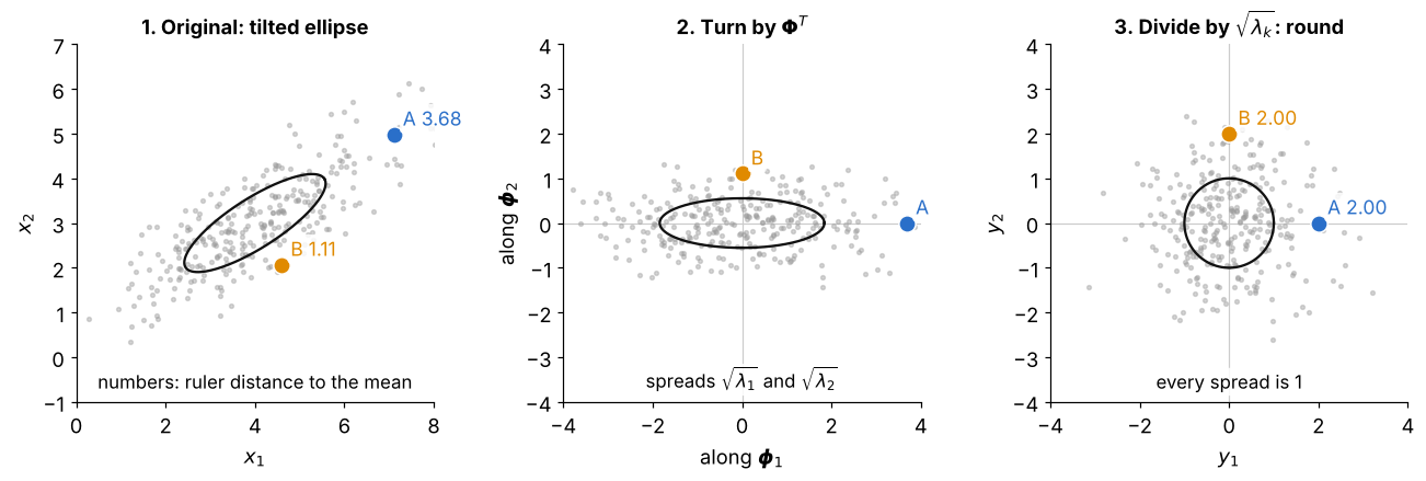
The three panels are the steps of :
- left: the tilted cloud; the black ellipse is one spread from the mean; A and B each lie two spreads out, A on the long axis and B on the short one
- middle: only turns, so the ellipse lines up with the axes, with spreads and , and the features become uncorrelated
- right: dividing by squeezes the long axis and stretches the short one, so the covariance becomes and the ellipse a circle
- A was from the mean and B only , but after whitening both are : distances are now in units of the cloud's own spread
Visual 2: what a too small eigenvalue does
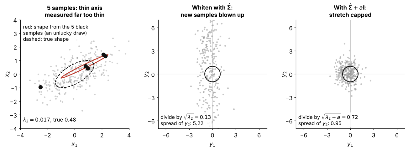
How to read it:
- left: 5 training samples that happen to lie almost on a line (an unlucky draw, picked on purpose) give along , while the true variance there is
- middle: whitening new samples of the same class with this divides by , so their spread along is instead of 1 and they look far from their own class
- right: with () the divisor is , so the stretch is capped; adding also slightly shrinks the long axis, so the cloud is a little narrower than the circle along
- this is the small-eigenvalue problem and its first fix in one picture