Introduction
PCA ended with eigenvectors of the covariance matrix. Eigen-decomposition writes the whole covariance matrix using its eigenvectors and eigenvalues. It explains why the PCA features are a good new set of axes: along the eigenvectors the features stop being correlated. It also gives PCA a compact trace form and shows what PCA keeps and what it can lose.
Main idea
For a symmetric $\boldsymbol{\Sigma}$, the unit eigenvectors are orthonormal, so $\boldsymbol{\Phi}^T\boldsymbol{\Phi}=\mathbf{I}$. Writing all $\boldsymbol{\Sigma}\boldsymbol{\phi}_i=\lambda_i\boldsymbol{\phi}_i$ at once gives $\boldsymbol{\Sigma}\boldsymbol{\Phi}=\boldsymbol{\Phi}\boldsymbol{\Lambda}$, so $\boldsymbol{\Sigma}=\boldsymbol{\Phi}\boldsymbol{\Lambda}\boldsymbol{\Phi}^T$ and $\boldsymbol{\Lambda}=\boldsymbol{\Phi}^T\boldsymbol{\Sigma}\boldsymbol{\Phi}$. The rotated data $\mathbf{Y}=\boldsymbol{\Phi}^T\mathbf{X}$ has covariance $\boldsymbol{\Lambda}$: uncorrelated features whose variances are the eigenvalues.
Overview
The whole note is one matrix identity, with every matrix :
Steps 1 to 4 build it, step 5 draws it in 2-D, step 6 uses it on the data, and step 7 uses it to write PCA as a trace.
Step 1: definition
The eigenvalues and eigenvectors of an matrix are defined by:
In words: multiplying most vectors by both stretches and turns them, but an eigenvector keeps its direction and is only stretched by the factor .
For a covariance matrix, multiply both sides on the left by a unit : , the variance of the data along . Keep this meaning in mind for every step below.
Step 2: symmetric means orthonormal
If is symmetric (, which every covariance matrix is), then eigenvectors of distinct eigenvalues are orthogonal. The proof uses only the definition, , and .
Take each eigenvector with unit length. Then:
Orthogonal plus unit length is called orthonormal.
Equal eigenvalues need care. The proof needs , so it says nothing about two eigenvectors that share one eigenvalue. This case is common: when , has at least eigenvalues equal to zero. For a symmetric matrix, the eigenvectors of a repeated eigenvalue can still be chosen orthonormal, so a full set of orthonormal eigenvectors always exists. They form a complete new set of perpendicular axes, a rotation of the original axes.
Questions to think about, using "eigenvalue is the variance along its eigenvector":
- if in 2-D, what shape is the cloud, and which directions are eigenvectors?
- if , what does the data look like along ?
Step 3: eigenvector matrix
Put the eigenvectors side by side as the columns of one matrix:
Entry of is row of times column of , which is . By Step 2 this is 1 on the diagonal and 0 elsewhere, so:
Why each step follows:
- says undoes , so is the inverse of
- a matrix times its inverse gives in either order, so as well
Step 4: decomposition
Put the eigenvalues on the diagonal of a matrix :
Now write all eigen-equations at once:
- column of is
- column of is , because is diagonal and only scales each column
- so for every is the single equation
Then use Step 3:
- multiply on the right by and use :
- multiply on the left by and use :
Multiplying out column by row gives the same thing as a sum, one piece per axis:
What each piece means: projects any vector onto axis , keeping only its part along . So says the covariance is a spread-weighted sum of projections onto its own axes.
Step 5: 2-D picture
For two dimensions:
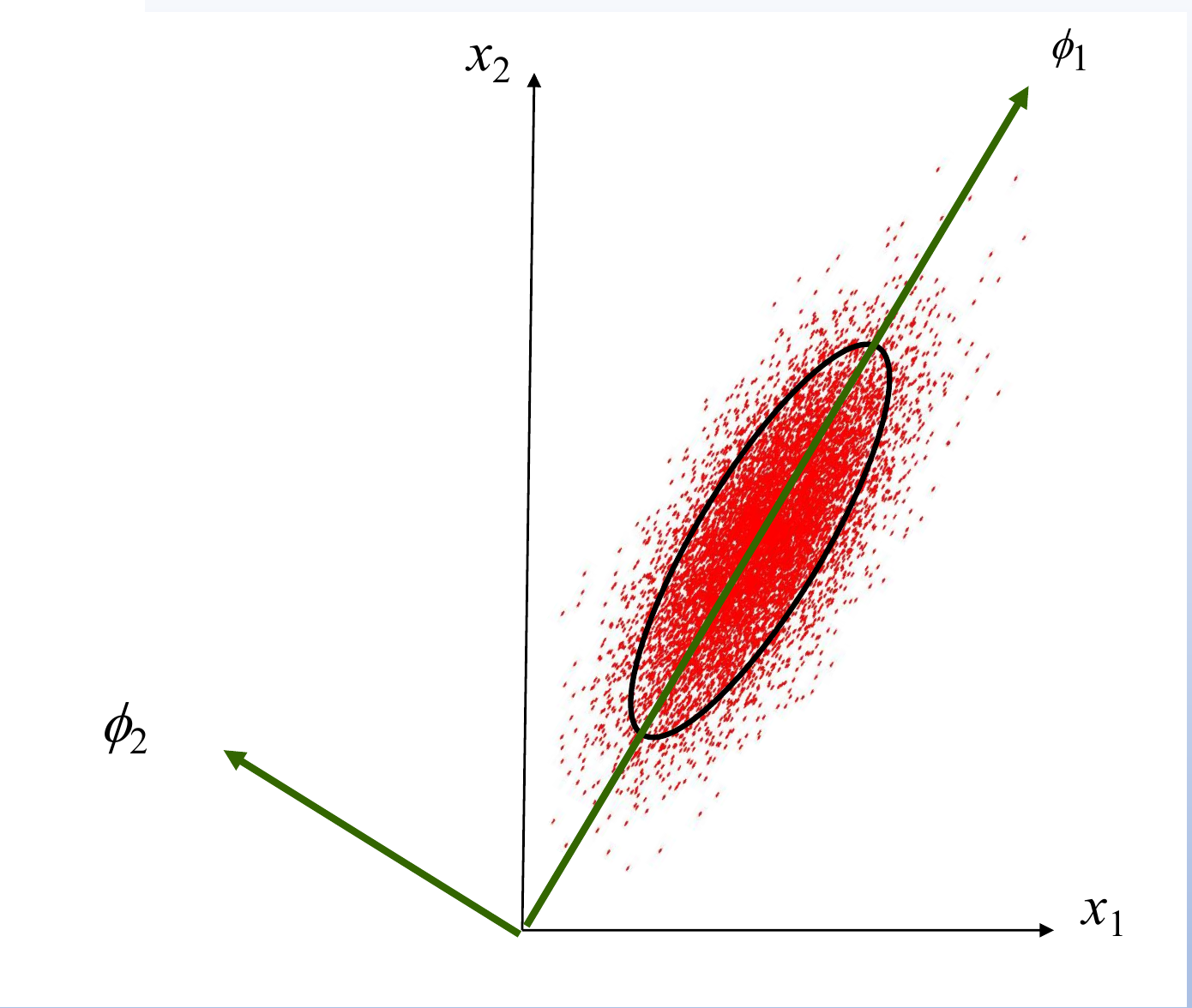
Here is entry of the covariance matrix: and are the variances of and , and is their covariance (Step 4 of Principal Component Analysis).
Reading the figure:
- the red cloud is samples of a 2-D Gaussian whose and are correlated, so
- the black ellipse is a contour of the cloud (a line of equal density), so its long and short axes show where the cloud is widest and thinnest
- the axes are drawn from the origin of , and for centred data the mean sits at the origin, so they pass through the mean
- points along the long axis of the ellipse, the direction of the largest variance
- is perpendicular to , along the short axis, with the smaller variance
- the eigenvectors are the original axes rotated to line up with the cloud
Step 6: rotated features are uncorrelated
Take the centred data matrix (one sample per column) and project every sample onto every eigenvector at once:
is just another name for the transform matrix . Write the covariance as . The factor is left out of both and , which changes nothing below. Then:
Explaining each equals sign:
- the first is Step 4
- the second puts in
- the third uses , so
- the fourth is the definition
- the last holds because is centred (each feature has mean zero, since the do), so is the covariance of the new features, in the same way as is for the old ones
What this means:
- the covariance matrix of the new features is the diagonal matrix
- every covariance between two different new features is zero, so the new features are uncorrelated
- the variance of feature is , which matches "eigenvalue is the variance" in PCA
- uncorrelated features share no linear information, so each one can be kept or dropped on its own, judged by its own variance (uncorrelated is weaker than independent, except for Gaussian data, where the two are the same)
- the cloud itself does not change, only the axes used to describe it
Step 7: PCA in trace form
The trace of a square matrix is the sum of its diagonal entries. Now let hold only the kept eigenvectors of , so it is (for example ). By Step 4, entry on the diagonal of is , the variance kept along direction . So PCA keeps the largest total variance in the -dimensional subspace:
where are the eigenvalues of , sorted from largest to smallest. The constraint is the -direction version of . Without it, longer columns would make the trace as large as you like.
With all eigenvectors, , using . So the total variation is the sum of all eigenvalues: PCA keeps and loses , which is the reconstruction error in PCA Reconstruction.
What PCA does well:
- it is an unsupervised method that minimizes the reconstruction error, which is the same as maximizing the variation in the reduced subspace, using variance as the measure of the information carried by the data
- the reduction lowers the computational cost of the later processing
What PCA can lose:
- any information lost may reduce the accuracy of the later processing
- the lost information, though less important for representing the data, could be critical for telling which class a sample belongs to
Why do we need this
It explains what PCA really does: rotate the axes to line up with the data's ellipse, so the features become uncorrelated, then drop the axes with the least variance. It also sets up the trace form that LDA changes.
Next step
The last point is a real problem for classification. Scatter Matrices shows why, and splits the spread into a part inside each class and a part between the classes.
Visual 1: turn, stretch, turn back
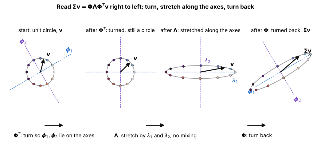
What does to the unit circle, read right to left; the coloured dots show where each point goes:
- only turns: the circle stays a circle, and , now lie on the coordinate axes
- is diagonal, so it stretches each axis by its own and mixes nothing: in these axes there is no covariance, as in Step 6
- turns back, so the stretched ellipse ends up lying along and
- so of Step 4 says a covariance is just a stretch along its own eigenvectors
Visual 2: covariance as a sum of flat pieces
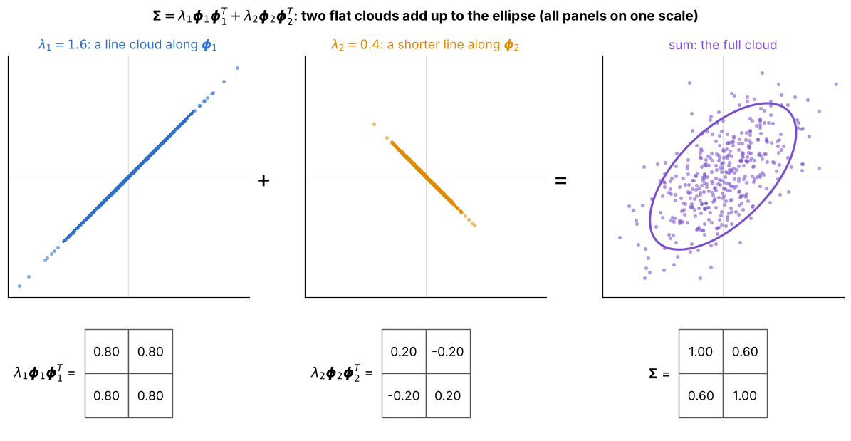
The covariance (the apple data of Projection onto an Axis) split into its two pieces, all panels on one scale:
- left: is the covariance of a cloud squashed onto the line of , with variance along it
- middle: is a shorter line cloud along , with variance
- right: adding the two grids entry by entry gives , and adding the two spreads gives the full ellipse
- this is at the end of Step 4