Introduction
PCA uses the spread of all the data together and ignores the class labels, so it can keep a direction along which the classes overlap. To choose directions for classification, the spread has to be split by class: how much the samples spread inside their own class, and how far the class centres are from each other. The scatter matrices measure these two parts. They are the building blocks of linear discriminant analysis.
Main idea
The within-class scatter $\mathbf{S}^w$ is the weighted average of the class covariances. The between-class scatter $\mathbf{S}^b$ is the weighted covariance of the class means around the overall mean. Together they make the total scatter: $\mathbf{S}^t=\mathbf{S}^w+\mathbf{S}^b$. Along a unit direction $\boldsymbol{\phi}$, a good direction for classification has a large $\boldsymbol{\phi}^T\mathbf{S}^b\boldsymbol{\phi}$ and a small $\boldsymbol{\phi}^T\mathbf{S}^w\boldsymbol{\phi}$.
Overview
All three matrices are covariance-like matrices, and they fit together as:
Step 1: problem of PCA for classification
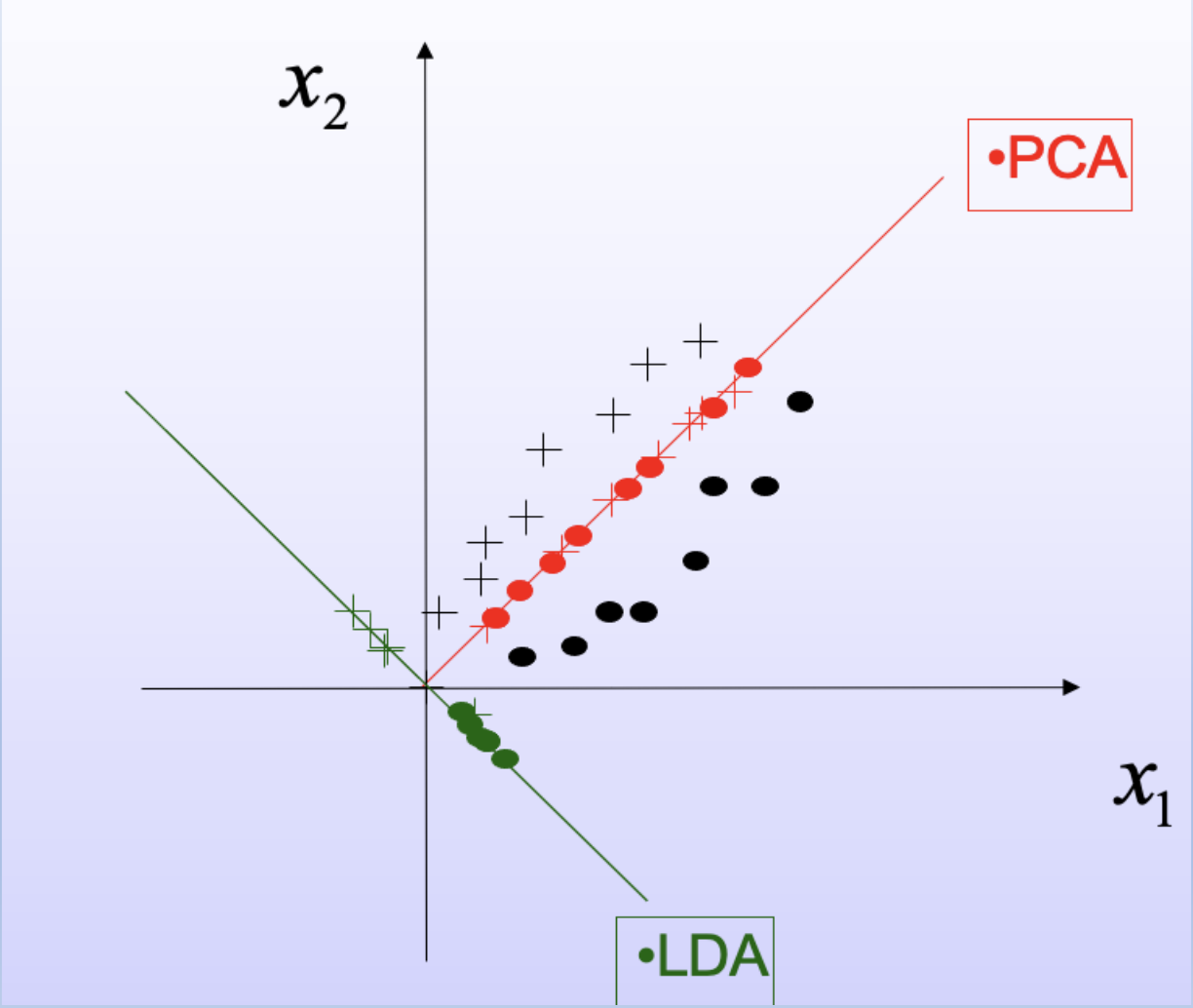
Reading the figure:
- the two classes ( and ) are both long and thin, and lie side by side along the same long direction
- PCA projects onto the direction of the largest total variance (red), which is that long direction
- after this projection the two classes land on top of each other, so they cannot be told apart
- the LDA direction (green) has less total variance, but after projecting onto it the two classes stay apart
- both lines are drawn through the origin, and only their direction matters for the projection
So the direction that represents the data best can be a poor direction for classification. The desired properties of a projection direction for classification are:
- maximize the separation between the projected class means
- minimize the projected within-class scatter (variance)
To score a direction on these two properties, the spread must be measured class by class. That is what the scatter matrices do.
Step 2: class mean and covariance
There are training samples of dimensions from classes, named . Class has samples, , so .
The mean and covariance matrix of class use only the samples of that class:
How to read them:
- means "add over the samples that belong to class "
- is built the same way as in PCA, with the class mean in place of the overall mean
- so is the variance of class alone along
- as with in PCA, the centred samples of class can be put side by side as the columns of an class data matrix, and can be written with it in the same way as with
Step 3: within-class scatter matrix
What it is:
- a weighted average of the class covariances, where the weights add up to 1
- a bigger class counts more, in proportion to its number of samples
- it measures how spread out each class is around its own mean, which is the spread that makes classes hard to separate
Step 4: between-class scatter matrix
First, the overall mean. Group the sum over all samples class by class, and use :
So the overall mean is the weighted average of the class means. Then:
What it is:
- shrink each class down to one point, its mean , with weight
- is the covariance of these points around the overall mean
- it measures how far apart the class centres are, which is the spread that helps classification
Step 5: trace as total variation
The trace (sum of the diagonal) of a covariance matrix adds up the variances of all features, because each diagonal entry is the variance of one feature (Step 4 of Principal Component Analysis). So it turns a whole matrix of spread into one number:
- is the total variation amount of all samples
- is the total variation amount of samples within classes
- is the total variation amount of samples between classes
Step 6: total equals within plus between
Proof, step by step:
- split each sample's offset from the overall mean into two parts, sample to class mean and class mean to overall mean:
- take the outer product of this with itself, which gives four terms: , two cross terms, and
- add over the samples of class : each cross term contains , so both cross terms vanish
- the first term adds up to , by the definition of
- the last term is the same for every sample in the class, so it adds up to
So for one class:
Add over all classes and divide by . The left side becomes , the first term becomes and the second becomes . In words: total spread = spread inside the classes + spread of the class centres.
Step 7: spread along a direction
Project onto a unit vector . As in PCA, is the variance along for any of these matrices:
- is how far apart the projected class means are, so the first desired property wants it large
- is how spread out each projected class is, averaged over the classes, so the second desired property wants it small
- is what PCA maximizes
This shows the problem of Step 1 in symbols: a large can come from the unhelpful within-class part, and PCA cannot tell which.
Why do we need this
The scatter matrices turn "class means far apart, each class tight" into numbers that can be optimized. They are all a classification-minded feature extractor needs to know about the training data.
Next step
Linear Discriminant Analysis uses and to find the directions that separate the classes best.
Visual 1: one offset split in two
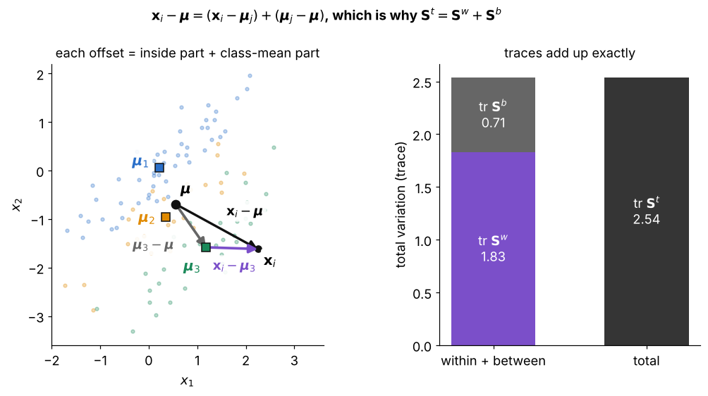
Three classes with 50, 25 and 35 samples:
- for one sample of class 3, the black offset is the purple step inside the class plus the grey step from the overall mean to the class mean
- the purple steps of a class add to zero, so the cross terms vanish when the outer products are summed, which is the proof in Step 6
- right: the traces computed from the data, , so total variation is within-class plus between-class
- is not the centre of the three class means here, because it weights each mean by its class size
Visual 2: within and between along each direction
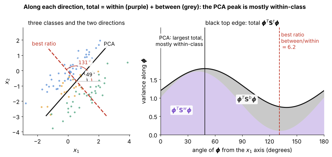
Left, the same three classes with the two directions and their angles; right, the unit vector turned through every angle:
- purple is , grey is , and the black top edge is their sum
- PCA picks the top of the black curve at , along the long side of every class, but that height is almost all purple, the spread that hurts classification
- the ratio of grey to purple is largest at , across the classes, a direction PCA would rank low
- this is Step 7 in a picture: a large total spread can come from the unhelpful within-class part