Introduction
Linear Discriminant Analysis needs , but with fewer samples than dimensions is singular. LDA variants are the ways around this. Each one moves to a smaller subspace where the matrices it needs are well behaved, or changes the criterion so that no impossible inverse is needed.
Main idea
With $q$ samples and $c$ classes, the data only fill a $(q-1)$-D range space of $\mathbf{S}^t$, and $\mathbf{S}^w$ only covers $q-c$ of those directions. Each variant picks a subspace from this picture and runs an LDA-like criterion there. All of them extract the discriminative information on the training data (DT) or remove the redundant information on the training data (RT), which is the same job a classifier does.
Overview
Every variant works in a subspace of the -D data space. The range space of a matrix is the set of directions where it has nonzero eigenvalues (Step 1 defines it fully), and its size is the rank. The sizes below take each rank at its upper limit, which is the usual case when there are fewer samples than dimensions:
How the spaces sit inside each other:
- all training data lie in the -D range space of , so nothing outside it matters
- inside it, the -D range space of holds the directions with some within-class spread, and it lies inside the range space of because and neither part can be negative along any direction, so a direction with zero total spread also has zero within-class spread
- the remaining directions have zero within-class spread but some total spread, so there all the spread is between the classes
- the -D range space of , where the class means differ, also lies inside the range space of , and it has the same size as the space in the previous bullet, but in general it is a different space
Step 1: words for subspaces
For a covariance-like matrix, sort its eigenvectors by eigenvalue. Then:
- the range space is spanned by the eigenvectors with nonzero eigenvalues, the directions where the data actually spread
- the null space is spanned by the eigenvectors with zero eigenvalue, the directions with no spread at all
- the principal space is spanned by the eigenvectors with the largest eigenvalues
- a complement space is what is left of a space after removing a subspace from it
A matrix can be inverted inside its range space, because there all its eigenvalues are nonzero.
How to compute a matrix inside a subspace:
- take orthonormal vectors that span the subspace, as the columns of an matrix
- project every sample onto them, , which gives -dimensional data
- the scatter matrix of the projected data is the matrix , by the same steps as in PCA with in place of
- a tilde, hat or bar on a scatter matrix, such as , or , marks the matrix computed this way inside the chosen subspace
- the mark only says which subspace is used: it is unrelated to the tilde on a centred sample , and in PCA + LDA and in DLDA are computed in different subspaces
Step 2: map of the variants
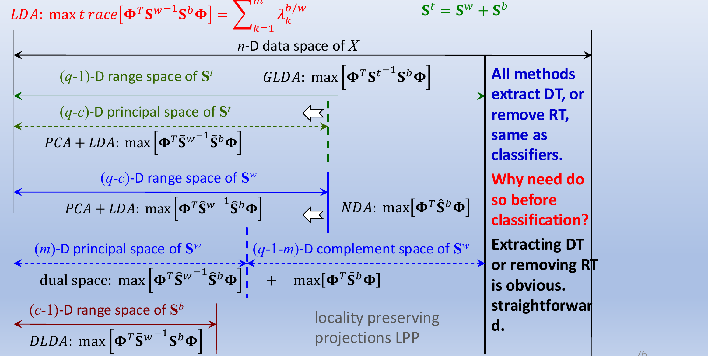
How to read the figure:
- each horizontal arrow is one subspace, labelled with its dimension
- the formula under or beside an arrow is the variant that works in that subspace
- the top line is plain LDA in the full -D space, together with
- solid arrows are range spaces and dashed arrows are principal spaces, and the white arrows mark where a space is cut down to a smaller one
- the length of an arrow shows only the size of the space, so the range space of drawn at the left does not mean it sits inside the range space of
| Method | Works in | Criterion |
|---|---|---|
| LDA | -D data space | |
| GLDA | -D range space of | |
| PCA + LDA | -D principal space of | |
| PCA + LDA | -D range space of | |
| NDA | -D part of the range space of outside the range space of | |
| Dual space | -D principal space of , plus its -D complement | |
| DLDA | -D range space of |
Step 3: each variant explained
GLDA (generalized LDA):
- replaces with , which has the larger rank , so it can be inverted in its -D range space
- along one direction, , where is the Fisher ratio (divide the top and bottom by and use ), and this grows whenever grows, so when can be inverted GLDA picks the same directions as LDA
PCA + LDA, two versions:
- first reduce the data to dimensions, either with the eigenvectors of with the largest eigenvalues (principal space of ) or with the eigenvectors of with nonzero eigenvalues (range space of )
- why and not : inside the -D range space of , still has rank only , so it is still singular there
- in the range space of , has no zero eigenvalues by construction, and in the principal space of , usually has none, so it can be inverted
- then run ordinary LDA there
NDA (null space discriminant analysis):
- works in the directions that are inside the range space of but outside the range space of , which is the null space of where the data still spread
- there the within-class scatter is zero, so every class collapses to a single point
- the Fisher ratio has a zero bottom, so it only maximizes the between-class scatter
Dual space:
- splits the -D range space of into the -D principal space of and its -D complement, where is the chosen size of this split, not the number of output features
- runs ordinary LDA in the principal space, where can be inverted
- maximizes the between-class scatter alone in the complement, where the within-class scatter is small or zero
- adds the two, so no direction is thrown away
DLDA (direct LDA):
- starts from the -D range space of , where all the differences between class means live
- computes inside it and runs LDA there, so it gives at most features
LPP (locality preserving projections) is named as another method in this family, without its details.
NDA and the small-eigenvalue problem point in opposite directions:
- NDA trusts zero within-class spread: if the classes truly do not spread in a direction, that direction separates them perfectly
- Discriminant Function in Eigenspace distrusts it: with few samples, zero spread is often an accident of these particular samples, and new samples of the same class do spread there
- the training data alone cannot tell the two cases apart, which is the question Objectives of Dimensionality Reduction takes up
Step 4: DT and RT
Two kinds of information on the training data:
- DT is the discriminative information on the training data
- RT is the redundant information on the training data
All these methods extract DT or remove RT, the same job a classifier does. Extracting DT or removing RT is obvious and straightforward, and a proper classifier already does it. So the real question is: why do it before classification at all?
Step 5: summary of PCA and LDA
What each method extracts:
- PCA extracts the most representative information on the whole data
- LDA extracts the most discriminative information under a linear constraint, which means the features can only be linear projections
| Property | PCA | LDA |
|---|---|---|
| uses class labels | no | yes |
| criterion | ||
| directions | eigenvectors of , orthonormal | eigenvectors of , not orthogonal in general |
| most useful features | ||
| keeps | most representative information | most discriminative information |
It is widely believed that discriminative information is the most important for recognition, so almost all researchers prefer LDA to PCA for recognition. Numerous efforts were made in the 1990s to 2010s to make LDA workable.
Why do we need this
Real image data almost always has more pixels than training images, so plain LDA almost never runs as written. These variants are how LDA is used in practice, and they all come from the same picture of ranks and subspaces.
Next step
Objectives of Dimensionality Reduction answers why dimensionality reduction is done before classification.
Visual 1: nested subspaces and where each variant works
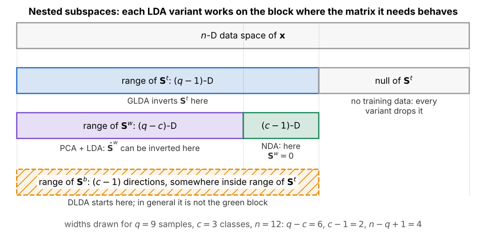
Each bar is a set of directions in the -D data space, drawn to scale for , , :
- the range of ( directions) holds all training data, and its null space holds none, so every variant drops it
- inside it, the range of ( directions) is where PCA + LDA can invert the within-class scatter
- the green block ( directions) has total spread but zero within-class spread, so this is where NDA works
- the range of also has directions inside the range of , but in general it is not the green block; DLDA starts from it
Visual 2: NDA in two dimensions
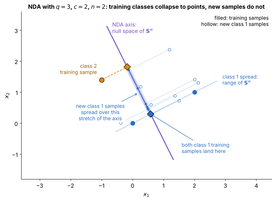
The smallest case with a null space: samples, class 1 has two and class 2 has one, in :
- the range of is the dotted line through the two class 1 samples, the only direction where class 1 spreads
- the NDA axis is perpendicular to it, the null space of , and there both class 1 training samples land on one point (blue diamond) and class 2 on another (orange diamond)
- each training class is a single point on the NDA axis, so the within-class scatter is zero and only the gap between the classes counts
- the hollow circles are new class 1 samples: their projections cover a whole stretch of the NDA axis (blue band), which is the warning that zero spread can be an accident of few samples