Introduction
Principal Component Analysis found the best single direction. In practice you keep directions: the eigenvectors of the largest eigenvalues of . This note builds the -dimensional transform, rebuilds the sample from it, shows that the error is exactly the sum of the dropped eigenvalues, and finds how many eigenvalues can be nonzero.
Main idea
$\mathbf{y}=\boldsymbol{\Phi}^T(\mathbf{x}-\boldsymbol{\mu})$ and $\hat{\mathbf{x}}=\boldsymbol{\Phi}\mathbf{y}+\boldsymbol{\mu}$, where $\boldsymbol{\Phi}$ holds the eigenvectors of the $m$ largest eigenvalues of $\mathbf{S}^t$. Each dropped direction loses its own variance, so $E[\|\Delta\|^2]=\sum_{k=m+1}^{n}\lambda_k$. With $q$ samples, $\mathbf{S}^t$ has at most $q-1$ nonzero eigenvalues, so $q-1$ dimensions already rebuild the training data with zero error.
Overview
The sizes, with dimensions, kept directions and :
goes down from to numbers, and goes back up from to .
Step 1: reduce to m dimensions
Sort the eigenvalues of from largest to smallest, , and keep the eigenvectors of the first :
How to read it:
- row of is , so entry of is , the coordinate along direction
- so is the one-direction projection of Principal Component Analysis, done times at once
- is symmetric, and the eigenvectors of a symmetric matrix can always be chosen orthonormal (perpendicular to each other and of unit length), so , and Eigen-Decomposition shows why
This is the famous principal component analysis (PCA) transform from -dimensional to -dimensional .
Why the top eigenvectors are the best directions:
- the goal is the same as for one direction: keep the most total variance, with each kept direction of unit length and perpendicular to the others
- the best first direction is , the best second direction perpendicular to it is , and so on, each adding the next largest variance
- Eigen-Decomposition writes this goal as one trace, and its answer is the eigenvectors of the largest eigenvalues
Step 2: reconstruct the sample
To rebuild the original -dimensional sample from the numbers, walk steps along each kept direction and add back the mean:
The second form comes from multiplying by column by column: column of times entry of .
Going down and back up in one line:
Why this is not a perfect rebuild:
- , but is with rank only , so when
- keeps the part of inside the kept directions and drops the rest, the -direction version of
- only with all eigenvectors is , and then
With these directions, the total reconstruction error is the smallest possible:
Step 3: error equals the dropped eigenvalues
The reconstruction error of one sample is (the index is dropped for short):
To find its size, use all eigenvectors. They are orthonormal directions in dimensions, so together they are a complete set of axes, and any centred sample is the sum of its pieces along them:
Explaining each step:
- the reconstruction keeps the first pieces, so the error is the rest:
- square it: , summing and from to
- is when and otherwise, so every cross term vanishes and
- write for the average over all training samples, then is the variance along , which is (eigenvalue is the variance, in Principal Component Analysis)
So the mean squared reconstruction error is:
where the are sorted in descending order. What this means:
- each dropped direction adds its own variance to the error
- dropping the smallest eigenvalues gives the smallest possible error, which is why PCA keeps the largest
- the total error over all samples is , because is the average and is the sum
Step 4: rank of the total scatter matrix
The rank of a matrix is its number of independent columns, which is the number of independent directions its outputs can point in. For a symmetric matrix it equals the number of nonzero eigenvalues, because (Eigen-Decomposition) only gives outputs along the eigenvectors with .
Why the rank is at most :
- is , so its rank is at most
- for any vector , is a weighted sum of the (each is a number), so the outputs of cannot cover more directions than the vectors span
- the centred samples add up to zero:
- so the last one is fixed by the others, , and the vectors span at most directions
So has at most nonzero eigenvalues. For example, 2 samples always lie on one line through their mean, and 3 samples always lie in one plane, even in a space of thousands of dimensions.
What follows when :
- the eigenvalues are all zero, so the data has no spread at all along their eigenvectors
- PCA with a -dimensional fully represents the original -dimensional training data, because every dropped eigenvalue is zero:
Why do we need this
It turns PCA into a recipe with a dial: choose , and the eigenvalues tell you exactly how much is lost. The rank result also warns that with few samples, most directions in a high-dimensional space contain no training data at all.
Next step
Eigen-Decomposition writes the whole covariance matrix in terms of its eigenvectors, and shows why the PCA features are uncorrelated.
Visual 1: error is the sum of dropped eigenvalues
How to read it:
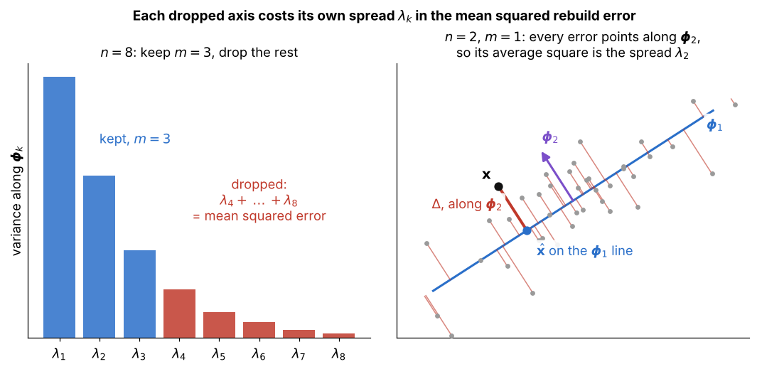
- left: the eigenvalues of for , sorted from largest to smallest, with kept (blue) and 5 dropped (red)
- right, a 2-D case with : each sample is rebuilt as on the line, and the error (red) always points along the dropped axis
- so is the squared coordinate along , and its average over the samples is the spread along , which is
- with more dropped axes the error has one such piece per dropped axis, at right angles, so the mean squared error is , as in Step 3
Visual 2: why few samples give few directions
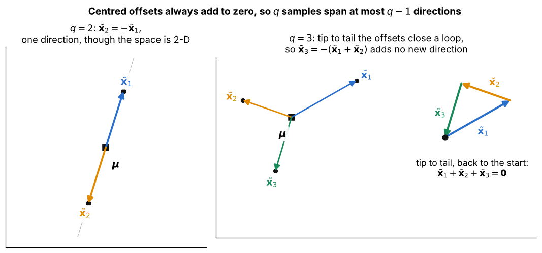
The cause behind the rank result of Step 4:
- left, : the two centred offsets are exact opposites, , so they point along one line even though the space is 2-D
- right, : laid tip to tail, the three offsets come back to the start, so adds no new direction
- this holds for any , because the offsets from the mean always add to zero, so samples span at most directions
- with samples in dimensions, only 5 directions hold any data, and the other 10 eigenvalues of are zero