Introduction
A Lagrange multiplier finds the best value of a function when the variables must stay on a constraint (the general idea is in Lagrange Multipliers). In Part 2 it appears at one key moment: it turns "find the direction of largest variance" into "find an eigenvector". Understanding why it works is understanding why PCA's answer is an eigenvector.
Main idea
At the best point on a constraint, you cannot improve by moving along the constraint, so the gradient of the function must point straight out of the constraint, parallel to the gradient of the constraint: $\nabla f=\lambda\nabla g$. In PCA, $f=\boldsymbol{\phi}^T\mathbf{S}^t\boldsymbol{\phi}$ and $g=\boldsymbol{\phi}^T\boldsymbol{\phi}=1$ give $\mathbf{S}^t\boldsymbol{\phi}=\lambda\boldsymbol{\phi}$, and the multiplier $\lambda$ turns out to be the variance kept.
What it is
To make as large as possible while keeping :
which is what you get by setting the gradient of to zero.
Physical meaning
Why the gradients must be parallel:
- the constraint is a surface you must stay on, so you can only move along it
- the gradient points in the direction where rises fastest
- if had any part along the surface, moving that way would raise , so you were not at the best point
- at the best point, has no part along the surface, so it points straight out of it, which is the direction of
What the multiplier means in PCA:
- turns out to be the value of itself, the variance kept, which is why it can be used to rank the candidates
What the other eigenvectors mean:
- every eigenvector is a flat point of the spread on the sphere of unit vectors: the largest, the smallest, and in more dimensions saddle points in between
- the second eigenvector is the best direction that is perpendicular to the first, the third is the best perpendicular to both, and so on
Why a constraint is needed at all:
- without , doubling multiplies by 4, so the "best" would be infinitely long
- we want a direction, so the length is fixed and only the direction is free
Where it is used
| Note, step | What the Lagrange multiplier does there |
|---|---|
| Principal Component Analysis, Step 5 | the best unit direction for must satisfy , so it is an eigenvector |
| Principal Component Analysis, Step 6 | the multiplier equals , the variance kept, so the largest wins |
| Eigen-Decomposition, Step 7 | the -direction version uses the constraint |
| Linear Discriminant Analysis, Steps 2 and 3 | the Fisher ratio does not change when is scaled, so no constraint is needed; setting its gradient to zero gives , the same form as a Lagrange answer with the constraint , which fixes the within-class spread to 1, so every direction is measured in within-class units |
Common traps
Points that are easy to get wrong:
- the Lagrange condition is met by every eigenvector, including the worst one; it only narrows the answer down to the eigenvectors, and the eigenvalue then picks the best
- the condition is also met at a minimum and at saddle points on the constraint, so you still have to check which candidate is the maximum
Test yourself
In PCA, why must the best direction be an eigenvector, in one picture?
The unit vector can only turn sideways. If had a sideways part, turning toward it would raise the variance. At the best direction it has none, so points along .
What does the multiplier equal in PCA, and why does that matter?
Multiplying by gives , the variance kept. So among all the eigenvectors, the one with the largest is the best.
Why do we need this
The Lagrange step is where an optimization problem becomes an eigenvector problem. Seeing it as "no sideways part of the gradient" explains why PCA's directions are eigenvectors without needing any eigenvector computation.
Visual 1: gradient parallel to the constraint normal
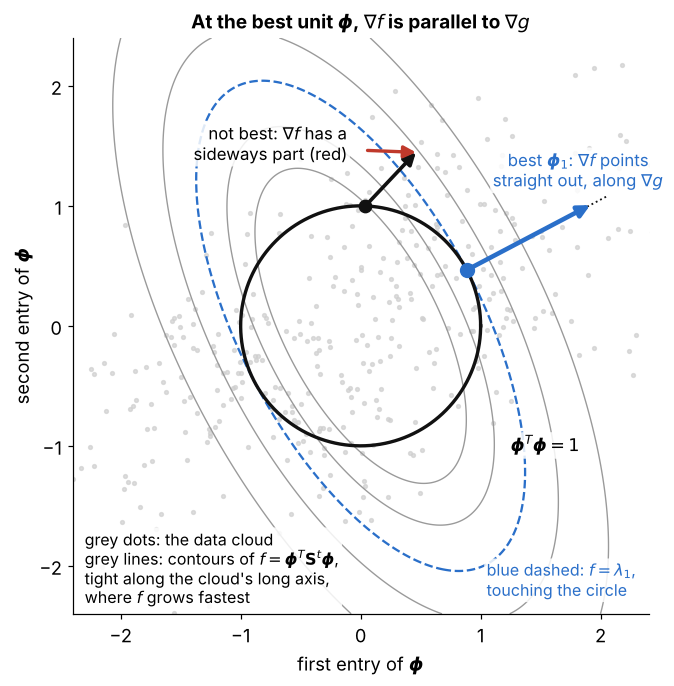
The axes are the two entries of a candidate unit direction , drawn over the data cloud (grey dots):
- the black circle is the constraint , and the grey lines are contours of
- the contours are tight along the cloud's long axis, because , the spread along , grows fastest when points that way
- at a point that is not best, has a sideways part along the circle (red), so turning that way would raise
- at the best point , points straight out of the circle, along , so ; there the contour just touches the circle
Visual 2: sideways push around the circle
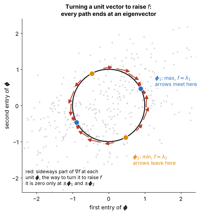
Each red arrow is the sideways part of at one unit , the way to turn to raise :
- the arrows vanish at exactly four points, and , where holds; these are the eigenvectors
- the arrows meet at : turning either way lowers , so this is the maximum,
- the arrows leave : it also has no sideways part, but it is the minimum,
- so the Lagrange condition only narrows the answer to the eigenvectors, and comparing their picks the best one