Introduction
The trace of a square matrix is the sum of its diagonal entries. For a covariance or scatter matrix, it turns a whole matrix of spread into one number: the total spread of the data. PCA and LDA are both written as "maximize a trace", so the trace is how the course scores a set of projection directions. The matrices it is applied to are explained in Covariance Matrix in Pattern Recognition.
Main idea
For a covariance matrix, $\operatorname{trace}(\boldsymbol{\Sigma})$ is the sum of the variances of all features, the total spread of the cloud. It also equals the sum of the eigenvalues, because turning the axes does not change the total spread. With $m$ orthonormal directions in $\boldsymbol{\Phi}$, $\operatorname{trace}(\boldsymbol{\Phi}^T\boldsymbol{\Sigma}\boldsymbol{\Phi})$ is the spread kept in those directions.
What it is
Physical meaning
For a covariance matrix :
- total spread: each diagonal entry is the variance of one feature, so the trace is the total variance of all features together
- average squared distance: adding the variances of all features gives , the average squared distance of the points from the mean
- independent of the axes: turning the axes does not change any distance (Pythagoras), so the trace is the same in any set of perpendicular axes, and in the eigenvector axes it is
- kept spread: with orthonormal columns in , entry on the diagonal of is , the variance along direction , so the trace is the total spread kept in the chosen directions
- kept plus lost is fixed: the total is split into what the chosen directions keep and what is thrown away
Where it is used
| Note, step | What the trace measures there |
|---|---|
| Scatter Matrices, Step 5 | , and are the total, within-class and between-class variation |
| Eigen-Decomposition, Step 7 | PCA maximizes , the kept variance, which is the sum of the top eigenvalues |
| PCA Reconstruction, Step 3 | the error is the total minus the kept part, the sum of the dropped eigenvalues |
| Eigenvalue Regularization, Step 2 | is the lost spread shared out equally over the dropped axes |
| Linear Discriminant Analysis, Step 1 | LDA wants a small within-class trace and a large between-class trace |
| Linear Discriminant Analysis, Step 4 | the LDA trace, at its eigenvector answer, adds up the Fisher ratios of the chosen directions; the trace form is a shorthand, since taken literally it has no length limit |
Common traps
Points that are easy to get wrong:
- maximizing a trace only makes sense with a length constraint such as ; otherwise longer columns make it as large as you like
- the LDA trace is not divided by , and it equals the sum of Fisher ratios only at the unit-length eigenvectors
Test yourself
Why is the trace of a covariance matrix equal to the sum of its eigenvalues?
The trace is the average squared distance of the points from the mean. Turning the axes does not change distances, and in the eigenvector axes the spreads along the axes are the eigenvalues.
In PCA, what are the kept and the lost parts of the total spread?
Kept: along the chosen eigenvectors. Lost: , which is the mean squared reconstruction error.
Why do we need this
The trace is how PCA and LDA turn "a good set of directions" into one number to maximize. Reading it as "total spread kept" makes both criteria a picture, not just a formula.
Visual 1: total spread does not depend on the axes
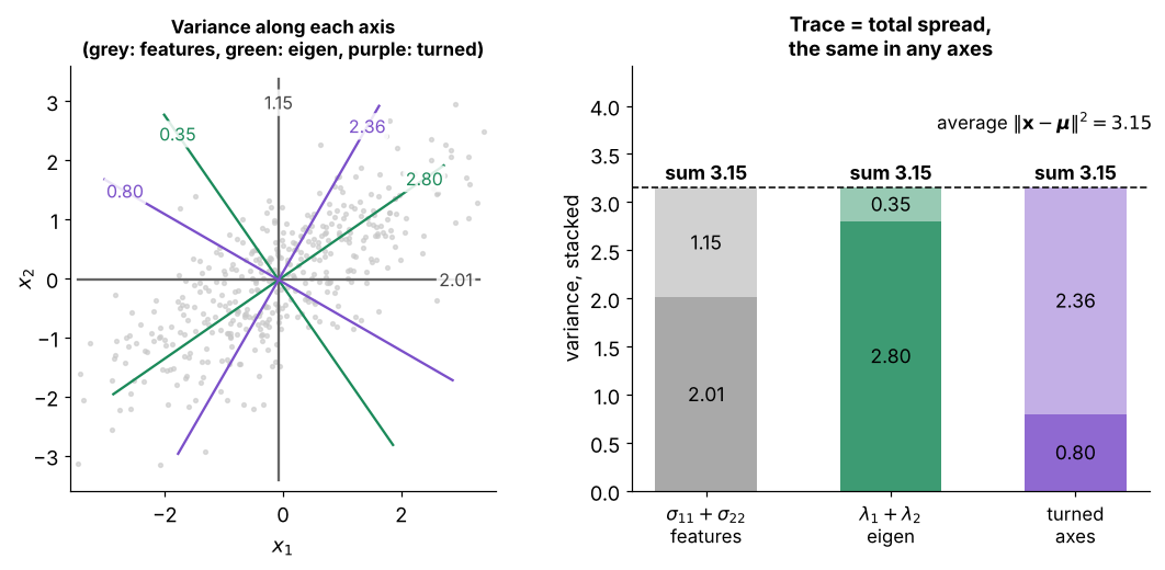
How to read it:
- left: one cloud with three sets of perpendicular axes (grey: the feature axes, green: the eigenvector axes, purple: a set turned by ), each labelled with the variance of the data along it
- right: each bar stacks the variances along its two axes, and all three add up to
- the first bar is , the diagonal of , and the second is
- the red line is the average of over the samples, the same , which is why turning the axes cannot change the trace
Visual 2: kept plus lost spread
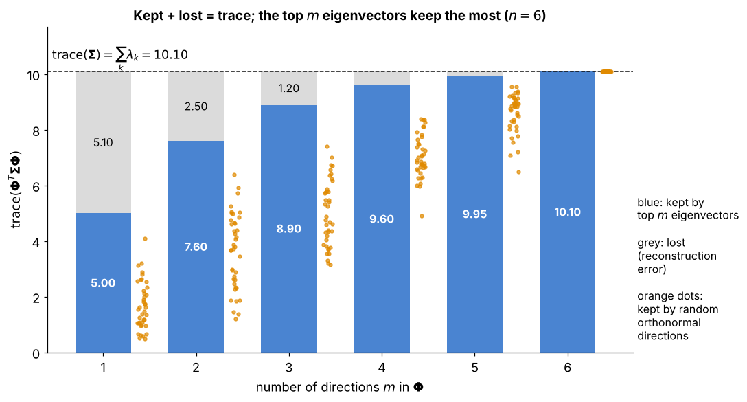
Here is with :
- blue is when holds the top eigenvectors, the sum of the top eigenvalues
- grey is what is lost, the sum of the dropped eigenvalues, which is the PCA reconstruction error
- orange dots use random orthonormal directions instead: they always keep less than the eigenvectors
- with all directions nothing is lost, and every choice keeps the full trace