Introduction
A covariance matrix describes the shape of a data cloud: how much each feature spreads, and how pairs of features move together. In pattern recognition it is the main way to describe a class, and every scatter matrix (, , ) is a covariance matrix of some set of points. Its eigenvectors and eigenvalues are explained in Eigenvectors and Eigenvalues in Pattern Recognition.
Main idea
$\boldsymbol{\Sigma}=E[(\mathbf{x}-\boldsymbol{\mu})(\mathbf{x}-\boldsymbol{\mu})^T]$ is an $n\times n$ symmetric matrix. Its diagonal holds the variance of each feature and its off-diagonal entries hold how pairs of features vary together. Put in any unit direction $\mathbf{a}$ and $\mathbf{a}^T\boldsymbol{\Sigma}\mathbf{a}$ gives the variance of the data along it, so for an ellipse-shaped cloud $\boldsymbol{\Sigma}$ describes its size, stretch and tilt.
What it is
How to read it:
- it is , one row and one column per feature
- the diagonal entry is the variance of feature , how much it spreads on its own
- the off-diagonal entry is the covariance of features and : positive if they tend to rise together, negative if one rises when the other falls, zero if they are uncorrelated
- , so is symmetric
- from samples, the expectation becomes an average over the samples, usually with (the ML estimate)
Physical meaning
What the matrix tells you about the cloud:
- shape: for Gaussian data, the points of equal density form ellipses (ellipsoids), and fixes their size, stretch and tilt
- variance along any direction: projecting onto a unit vector gives a 1-D feature with variance , so works like a machine that takes a direction and returns the spread along it
- tilt: nonzero off-diagonal entries mean the cloud is tilted against the feature axes; a diagonal means it is lined up with them
- size: the determinant is the product of the eigenvalues, so it grows with how much space the cloud covers; one tiny eigenvalue makes it almost zero, like a flat pancake with no volume
- inverse: squashes the cloud into a round ball, so it measures an offset in units of the cloud's own spread (Inverse Covariance and Whitening in Pattern Recognition)
Where the ellipse picture stops working:
- a class shaped like a banana or made of two separate clumps is not an ellipse, but it still has a covariance matrix, which then hides that shape
- this is why the nonparametric methods (Parzen window, kNN) and neural networks exist: they can follow class shapes that one mean and one covariance cannot
Three special shapes that the classifiers use:
- : a round cloud, the same spread in every direction
- diagonal : an ellipse lined up with the feature axes
- full : a tilted ellipse
Scatter matrices are covariance matrices
Each scatter matrix is the covariance of a different set of points:
- is the covariance of all samples together, ignoring the class labels
- is the average of the class covariances, the spread inside each class
- is the covariance of the class means around the overall mean, the spread between classes
- : total spread is spread inside the classes plus spread of the class centres
Where it is used
| Note, step | What the covariance matrix does there |
|---|---|
| Gaussian Discriminant Function, Steps 1 to 5 | describes the shape of class ; appears in the distance and in the bias |
| Quadratic, Linear and Minimum Distance Classifier | the three classifiers are three cases of : different for each class, shared, or |
| Gaussian ML Estimates, Step 5 | is estimated from samples by averaging the outer products of the offsets |
| Principal Component Analysis, Steps 4 and 6 | is the covariance of all data, and is the variance PCA keeps along |
| Eigen-Decomposition, Step 6 | in the eigenvector axes becomes diagonal, so the new features are uncorrelated |
| Scatter Matrices | and split the total spread into an unhelpful and a helpful part for classification |
| Discriminant Function in Eigenspace, Step 6 | a estimated from few samples has eigenvalues that are too small, which misleads the classifier |
| Gaussian Discriminant Function, Step 5 | gives a tight class a higher score, and a tiny eigenvalue raises it a lot |
Common traps
Points that are easy to get wrong:
- "uncorrelated" (zero covariance) is a property of a pair of features, not of one feature
- pooling the raw samples of several classes into one covariance includes the gap between the class means; a shared covariance must subtract each class's own mean first
- a covariance estimated from samples has rank at most , so it is singular whenever , and does not exist
- (sample against sample) and (feature against feature) are both sums of products, but only the second is a covariance; attention's is of the first kind, a similarity between tokens
Test yourself
What does a large positive say about the cloud?
Features 1 and 2 tend to rise together, so the cloud is a tilted ellipse that leans along the direction where both grow.
Why is the variance along ?
The projected feature is , a number with mean zero. Its square is , and averaging puts in the middle.
When does a Gaussian classifier become linear, in terms of the covariance?
When every class has the same . The quadratic term and the term are then the same for all classes and drop out.
Why do we need this
The Bayes classifiers, PCA, LDA and the small-sample fixes all start from a covariance matrix. Reading it as "the shape of the cloud" explains why the classifier boundaries curve or stay straight, why PCA keeps some directions, and why few samples give a misleading shape.
Visual 1: each cloud next to its matrix
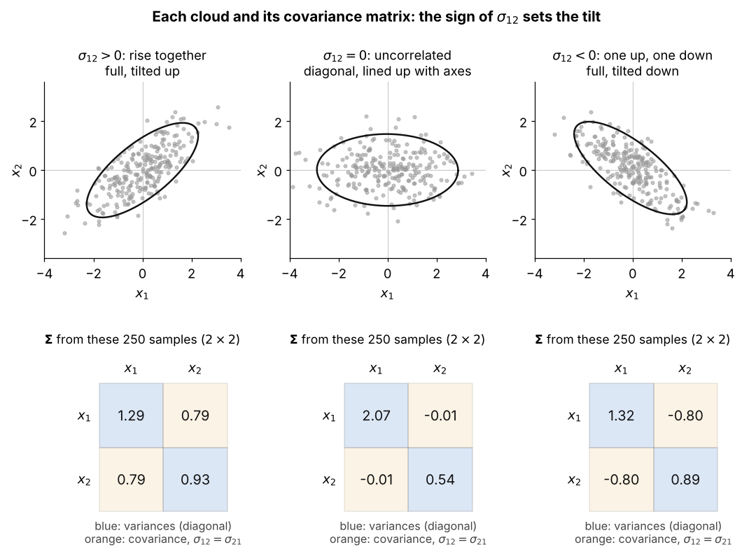
Each grid is computed from the 250 points drawn above it:
- rows and columns are the features ; the blue diagonal cells are the variances and the orange cells are the covariance
- : the cloud leans up to the right, : it leans down, : it is lined up with the feature axes
- in the middle cloud is about four times , so the ellipse is wide but not tilted (a diagonal )
- the off-diagonal from samples is never exactly zero ( here), since it is an average over a finite set
Visual 2: variance along any direction
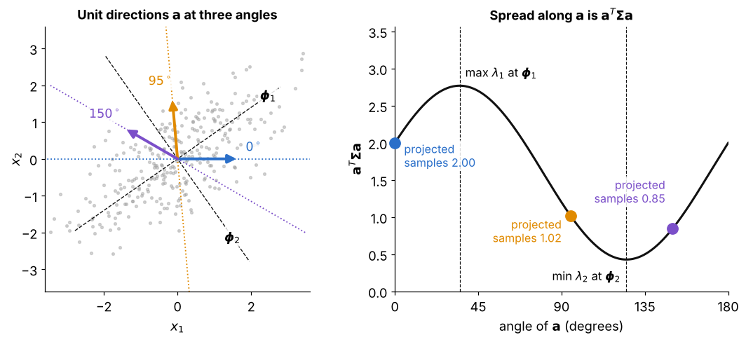
How to read it:
- left: three unit directions through the cloud, at the angles read on the right; the black dashed lines are the eigenvectors
- right: the black curve is as turns, and each dot is the variance of the samples actually projected onto that ; they match
- at the curve gives , which is just , the variance of feature
- the largest value is and the smallest is , reached at the eigenvectors, so is a machine that takes a direction and returns the spread along it
Visual 3: same matrix, different shapes
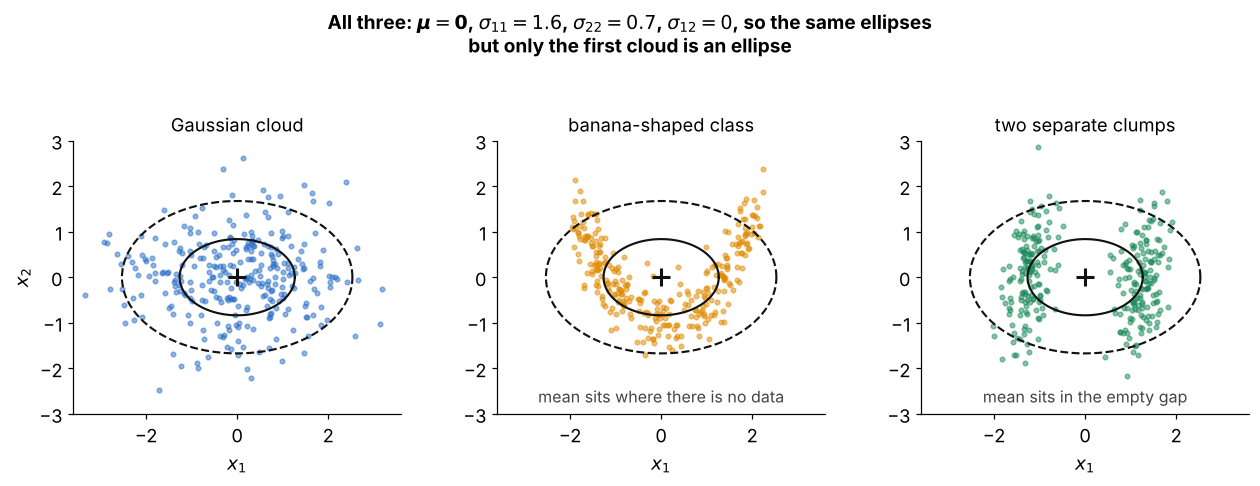
All three sets of points have exactly the same and :
- so they get the same ellipses (solid , dashed )
- only the left cloud really is an ellipse; the banana and the two clumps have their mean in a place with no data
- a Gaussian classifier using only and cannot tell these three classes apart
- this is the case where the ellipse picture stops working, and Parzen, kNN or a neural network is needed