Introduction
The gradient of a function of many variables is the vector of its partial derivatives (the general idea is in Gradient Vector). It points in the direction where the function rises fastest, and its length says how steep that is. Part 2 uses it in two ways: set it to zero to solve for the best values directly, or step against it again and again to train a network.
Main idea
$\nabla J$ points uphill on the error surface. At a best point the surface is flat, so $\nabla J=\mathbf{0}$; when that equation can be solved, it gives the answer in one go (mean, ML estimates, least squares, PCA, LDA). When it cannot, gradient descent walks downhill, $\mathbf{w}\Leftarrow\mathbf{w}-\eta\nabla J$, which is how LMS, backpropagation and every deep network learn.
What it is
Two kinds of gradient appear, and they mean different things:
- with respect to the input : of a discriminant points across the decision boundary, so for a linear classifier it is the boundary normal, such as
- with respect to the weights : says how to change the weights to lower the error, which is what training uses
Physical meaning
Picture the error as a landscape over the weights:
- direction: points uphill, the fastest way to make the error larger
- length: a long gradient means a steep slope, a short one means nearly flat
- flat point: at a minimum, a maximum or a saddle, so a zero gradient alone does not prove the best point
- one weight at a time: says how much the error changes if only moves a little
- shape of the bowl: for a squared error, the bowl's axes and steepness come from the eigenvectors and eigenvalues of , so along a direction with a tiny eigenvalue the bowl is almost flat, the weight there is poorly fixed by the data, and descent along it is slow
Two ways the course uses it:
- solve: set and solve, when the error is a simple bowl
- descend: when it cannot be solved, take small steps downhill, , with a small step size
Where it is used to solve directly
| Note, step | What setting the gradient to zero gives |
|---|---|
| Principal Component Analysis, Step 1 | the best single point for all samples is the mean |
| Principal Component Analysis, Step 5 | with the length constraint, the best direction is an eigenvector |
| Maximum Likelihood Estimation, Step 5 | the parameters that make the training data most likely |
| Gaussian ML Estimates, Steps 3 to 5 | the sample mean and the sample covariance with |
| Least Squares Single Layer Network, Step 4 | the least squares weights, |
| Linear Discriminant Analysis, Step 3 | the best direction for the Fisher ratio is an eigenvector of |
Where it is used to descend
| Note, step | What the gradient does there |
|---|---|
| LMS Gradient Descent Learning, Steps 1 to 3 | step downhill on the mean square error, one sample at a time |
| Backpropagation, Steps 5 to 7 | the chain rule passes the gradient back through the layers, giving each weight its own slope |
| Local Minima and Overfitting, Step 2 | the gradient is zero at a local minimum too, so descent can stop before the best weights |
| Activation Functions, and CNN as a Regularized MLP, Step 7 | the slope of the activation multiplies the gradient at every layer, together with the weights; ReLU passes it with slope 1 on active units and blocks it (slope 0) on inactive ones, while the sigmoid shrinks it by at most |
| CNN as a Regularized MLP, Step 5 | the gradient for a weight is proportional to the input it multiplies, so a shared weight gets a gradient from every position |
| Attention as Weighted Sum of Values, Step 3 | dividing by keeps the softmax away from regions where the gradient is almost zero |
Common traps
Points that are easy to get wrong:
- gradient descent moves against the gradient, with a minus sign
- a zero gradient can be a minimum, a maximum or a saddle point
- the gradient of is only when is symmetric
Test yourself
Why can the mean be found by setting a gradient to zero, but an MLP cannot?
The total squared distance to a single point is a bowl with one bottom, so has one simple solution. An MLP's error, with nonlinear activations between layers, has no such closed-form solution, so it is trained by walking downhill.
Why does a shared convolution weight learn from every pixel?
The gradient for a weight is proportional to the input it multiplies. A shared weight multiplies an input at every position, so its gradient is a sum over all positions.
Why does the sigmoid make deep networks hard to train?
Backpropagation multiplies the gradient by the slope of the activation at each layer. The sigmoid's slope is at most , so after many layers the gradient reaching the early layers is tiny.
Why do we need this
The gradient is the one tool behind both halves of Part 2. The statistical methods set it to zero to get their answers in closed form, and the neural networks follow it downhill because no closed form exists.
Visual 1: gradient arrows and descent on an error bowl
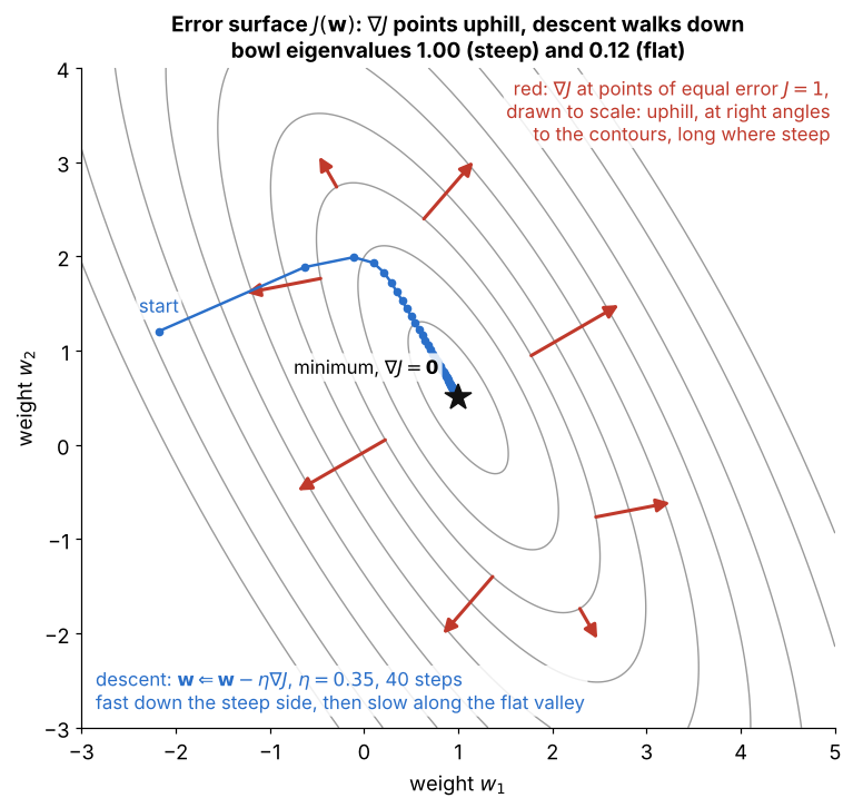
The grey ellipses are contours of a squared error over two weights:
- each red arrow is , drawn to scale, at a point with the same error : it points uphill and crosses the contour at a right angle
- the arrows are long on the steep sides and short at the two ends of the bowl, where it is nearly flat
- the blue path takes steps : it drops quickly down the steep side, then crawls along the flat valley
- the flat direction has the small eigenvalue , so the weight there is poorly fixed and descent along it is slow; at the star
Visual 2: effect of the step size
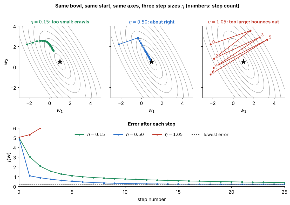
Same bowl, same start and same axes, only changes:
- : every step is safe but short, and after 25 steps the error is still well above the lowest value
- : the error falls fast and settles at the bottom
- : the numbered steps jump back and forth across the steep direction, each landing a little higher up, so the error grows
- a small step size is needed because the gradient only describes the surface near the current