Introduction
The MAP Decision Rule (maximum a posteriori: pick the class with the largest posterior) gives the best possible decision, but it needs the prior and the class-conditional PDF for every value of . In practice these are unknown, and the only thing available is a set of collected training samples. Statistical estimation, or machine learning, is the task of finding rules or values that describe a random variable , such as its PDF or the parameters of its PDF, from a set of training samples . Here is a vector of measurements, so is a PDF over numbers at once.
Main idea
Learn the prior $\hat{p}(\omega_k)=\frac{n_k}{n}$ by counting, and learn each class-conditional PDF from the samples of that class. A **nonparametric** approach (Parzen window, $k$-nearest neighbour) assumes no model and counts samples in a region. A **parametric** approach (maximum likelihood) assumes a model, such as a Gaussian, and only estimates its parameters.
Overview
The whole topic fills in the two unknowns of the MAP rule from data:
The prior is easy. Almost all the work is in estimating the PDF , and there are two ways to do it.
Step 1: what the best decision needs
The best decision, the one with the smallest probability of error, is:
Explaining each equals sign:
- is the probability of being wrong when deciding , which is the probability that the class is anything else,
- making smallest is the same as making largest
- by Bayes, , and is the same for every class, so it does not change which class wins
Names for the same thing: the MAP rule, the Bayes rule and the Bayes classifier all mean this best decision, and the Bayes error (or Bayes rate) is its error rate, the smallest error any classifier can reach.
To build an automatic pattern recognition system, the system must decide for any received , so it needs the PDF for all values of . In practice the PDF is unknown and can only be estimated from collected samples .
Step 2: what to learn
What is learned and why:
- the PDF is the complete information about a random variable
- it is difficult to estimate the posterior directly
- so we learn the prior and the class-conditional PDF instead
- the prior is one number per class, and each class-conditional PDF can be learned from the samples of its own class alone
Step 3: estimate the prior
The prior probabilities are estimated by counting:
where is the number of training samples of class and is the total number of training samples. It is the fraction of the training set that belongs to class , which is a good estimate when the training set has the same mix of classes as the real data.
Step 4: simplify the notation
The estimation method is the same for every class. So from here on:
- is written simply as , the PDF of one class
- means the number of training samples of that one class,
- the samples are drawn independently and identically distributed (i.i.d.) according to
What i.i.d. means:
- independent: one sample tells nothing about the next one
- identically distributed: every sample comes from the same PDF
Step 5: two approaches
| Approach | Assumption | Methods |
|---|---|---|
| Nonparametric | no model of the PDF | Parzen window, -nearest neighbour (kNN) |
| Parametric | the PDF has a known form with unknown parameters | maximum likelihood (ML) estimation of a multivariate Gaussian |
Notation
Letters used in this folder:
| Symbol | Meaning |
|---|---|
| number of dimensions of | |
| number of training samples of one class | |
| , | volume of a region, and side length (width) of a cell or kernel |
| number of samples inside a region, in the nonparametric notes | |
| , | parameter vector and its number of components, in the ML notes |
| number of classes, |
Letters that change meaning between notes:
- is the total number of samples when classes are counted (the prior here, and the kNN classifier), and the number of samples of one class when one PDF is estimated; the per-class count is then written or
- is the probability of a region in Nonparametric PDF Estimation, and an error rate in kNN Classifier, where is the Bayes error
- (not bold) is the class label of sample in kNN Classifier, and (bold) is the parameter vector in the ML notes
- the bar in means "given the class", and in it means "with the parameters set to "
- and both mean the training set
The letter is also used as a sample index () and a class index (), so check which one is meant from the context.
Reading order
The notes follow one line of thought:
- Nonparametric PDF Estimation: estimate by counting samples in a region,
- Parzen Window: fix the region size and count with a kernel, which turns into a smooth estimate
- k-Nearest Neighbour Estimation: fix the count and find the region size instead
- kNN Classifier: classify by a vote of the nearest samples, and how close it gets to the best error
- Maximum Likelihood Estimation: assume a model and pick the that best explains the samples
- Gaussian ML Estimates: for a Gaussian, the answer is the sample mean and the sample covariance
Concept map
flowchart TD
    A["Training samples D"] -->|"no model"| B["Nonparametric PDF estimation<br/>p̂(x) = k / (nV)"]
    B -->|"fix V, count k"| C["Parzen window<br/>average of kernels"]
    B -->|"fix k, find V"| D["k-nearest neighbour estimation"]
    D -->|"plug into MAP"| E["kNN classifier<br/>majority vote"]
    A -->|"model p(x|θ)"| F["Maximum likelihood estimation<br/>max Σ ln p(xₖ|θ)"]
    F -->|"Gaussian model"| G["Gaussian ML estimates<br/>sample mean and covariance"]
Why do we need this
Every classifier built later needs numbers that come from data. This folder gives the two basic ways to get a PDF from samples: count them directly, or fit a model's parameters.
Key math ideas
The math ideas this topic relies on, and where each one appears:
- Likelihood: the parameters are chosen to make the training set most likely, in Maximum Likelihood Estimation and Gaussian ML Estimates
- Gradient: setting the gradient of the log likelihood to zero gives the estimates, in Maximum Likelihood Estimation and Gaussian ML Estimates
- Covariance matrix: is estimated by averaging the outer products of the offsets, in Gaussian ML Estimates
- Softmax and posterior: the normalized kernel weights in the Parzen Window and the vote shares in the kNN Classifier act as posterior estimates
- Mahalanobis distance: the Parzen Window and the kNN Classifier use the plain Euclidean distance instead, which ignores the shape of each class
Visual 1: three estimates from one training set
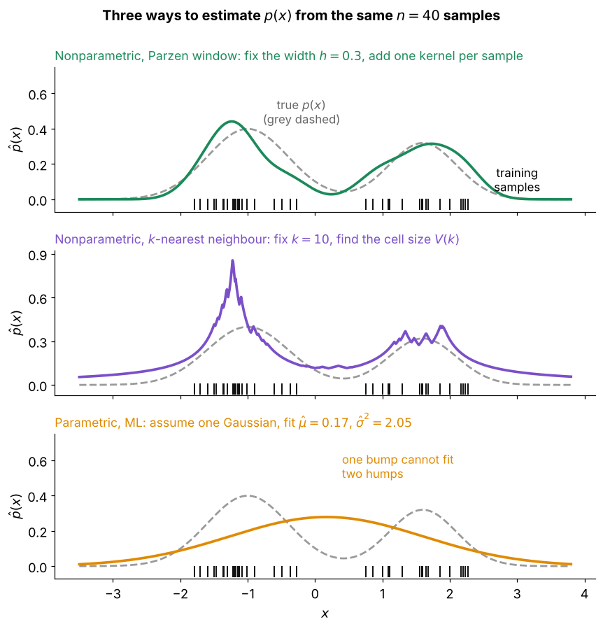
All three panels use the same samples (black ticks) from a two-humped true PDF (grey dashed):
- top, Parzen window: fix the width and put one bump on every sample, which gives a smooth estimate that follows both humps
- middle, -nearest neighbour: fix and let the cell grow, so it is sharp where samples crowd and never drops to zero in the tails
- bottom, maximum likelihood: assume one Gaussian and fit only and , so it is smooth but cannot show two humps
- nonparametric methods follow the data but are noisy, and a parametric method is stable but only as good as its assumed model