Introduction
The likelihood is a probability density read backwards: the measurement is fixed, and the question is which explanation makes it most probable. Part 2 uses it in two places that look different but are the same idea: choosing a class for a sample, and choosing parameters for a model. It also hides inside every squared error (the parameter case is in Maximum Likelihood Estimation).
Main idea
$p(\mathbf{x}|\cdot)$ read as a function of the unknown, with the data fixed, is the likelihood. As a function of the class, $p(\mathbf{x}|\omega_i)$ says how well each class explains $\mathbf{x}$; as a function of the parameters, $p(\mathcal{D}|\boldsymbol{\theta})$ says how well each parameter value explains the training set. Maximum likelihood picks the best explainer. Because it fits the very samples it is judged on, it tends to hug them, which is the root of the too-small spreads and of overfitting.
What it is
Two readings of the same kind of formula:
- over the classes: with fixed and varying, how likely this measurement is under each class
- over the parameters: with the training set fixed and varying, how likely the whole training set is for each parameter value
In both cases it is not a probability over the unknown: it does not add up to 1 over the classes or over .
Physical meaning
What it measures:
- "how well does this explanation account for what I saw"
- the class label plays the same role as a parameter: choosing the class with the largest likelihood is maximum likelihood over the classes, and it equals the MAP rule when the priors are equal
- the prior is what MAP adds on top: likelihood times prior is the top of the posterior
Why ML hugs the training data:
- ML chooses the parameters that make these particular samples as probable as possible
- a spread estimated this way is measured around a mean fitted to the same samples, so it comes out a little too small (the estimate)
- the same mechanism, much stronger, makes the smallest eigenvalues of a covariance estimated from few samples far too small
Squared error is a likelihood:
- if the target equals the output plus Gaussian noise, the log-likelihood of the training set is a constant minus the sum of squared errors
- so least squares, LMS and backpropagation with squared error are all maximum likelihood fits
- and the Gaussian log-density is times the Mahalanobis distance plus constants
Where it is used
| Note, step | What the likelihood means there |
|---|---|
| Prior, Likelihood and Posterior | is how likely the measurement is under class |
| MAP Decision Rule | with equal priors, the MAP rule picks the class with the largest likelihood |
| Gaussian Discriminant Function | the log-likelihood of a Gaussian class is the Mahalanobis distance plus terms in |
| Maximum Likelihood Estimation | the parameters are chosen to make the training set most likely |
| Gaussian ML Estimates | ML gives the sample mean and the sample covariance with , which is a little too small |
| Discriminant Function in Eigenspace, Step 6 | the smallest eigenvalues of an ML covariance are far too small, because they are fitted to the same few samples |
| Least Squares Single Layer Network | minimizing the squared error is maximum likelihood under Gaussian noise |
| Local Minima and Overfitting | fitting the training samples too closely is the network version of ML hugging its data |
Common traps
Points that are easy to get wrong:
- likelihood and posterior are different: against , and only the second adds up to 1 over the classes
- a density value can be larger than 1, so a likelihood is not a probability of the measurement
- the largest likelihood is not the best decision when the priors differ
Test yourself
When is "pick the class with the largest likelihood" the best rule?
When all priors are equal, since then likelihood times prior ranks the classes the same way as the likelihood alone.
Why does the ML covariance come out too small?
The mean is fitted to the same samples, so the samples sit a little closer to it than to the true mean. Dividing by corrects this on average.
Why is training with squared error a maximum likelihood fit?
If each target is the output plus Gaussian noise, the log-likelihood of the training set is a constant minus the sum of squared errors, so the smallest error is the largest likelihood.
Why do we need this
The likelihood links the two ways Part 2 learns from data: estimating densities and training networks. It also explains, in one mechanism, why estimates fitted to few samples look tighter than the truth.
Visual 1: likelihood as a function of the parameter
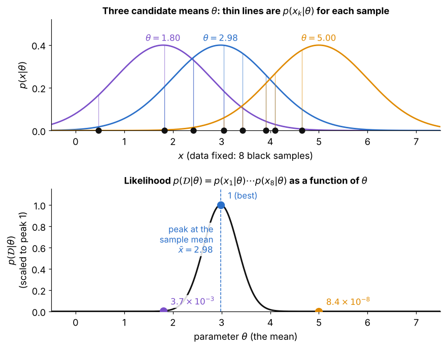
The 8 black samples are fixed, and only the candidate mean changes:
- top: for each candidate, the thin lines show , how probable each sample is under that Gaussian
- bottom: multiplying those 8 heights gives , plotted as moves
- the curve peaks at the sample mean ; moving to or makes the whole set far less likely
- this curve is not a density over : it is the same data read under different explanations
Visual 2: likelihood over the classes
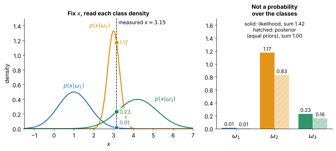
Here the measurement is fixed and the class changes:
- left: read off each class curve at ; the narrow class gives , more than 1
- right: the three likelihoods add up to , so they are not probabilities of the classes
- with equal priors, dividing by their sum gives the posteriors, which do add up to 1, and the winner is the same class
- with different priors the ranking can change, which is the gap between maximum likelihood and MAP
Visual 3: why ML hugs its samples
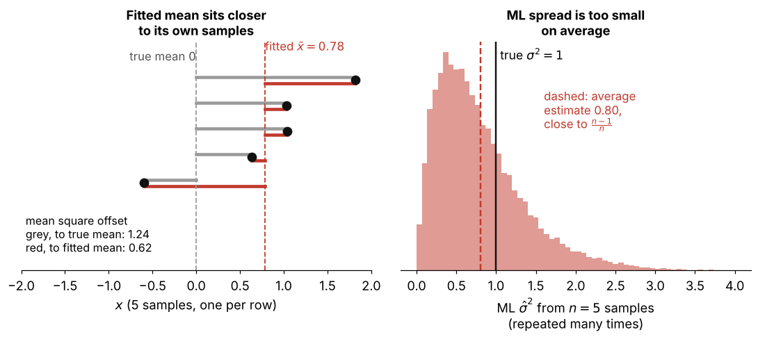
How to read it:
- left: one set of 5 samples from a class with true mean and variance 1, picked so that its fitted mean is clearly off
- the red offsets to are shorter on average than the grey offsets to the true mean ( against in squares), since is fitted to these very samples
- right: repeating this with many sets, the ML variance estimate from samples averages , not the true
- is , and the same pull makes the smallest eigenvalues of a covariance from few samples far too small