Introduction
-nearest neighbour (kNN) estimation is the second nonparametric way to estimate a PDF. The Parzen window fixes the size of the region and counts the samples. kNN does the opposite: it fixes the number of samples and lets the size of the region change.
Main idea
$\hat{p}(\mathbf{x})=\frac{k}{nV(k)}$: grow a region around $\mathbf{x}$ until it just encloses $k$ samples. The volume is small where samples are dense, so the estimate is high there, and large where samples are sparse, so the estimate is low there.
Overview
Both methods use the same formula, , and differ only in which number is fixed:
The bracket shows what depends on what: is the count found in a fixed volume, and is the volume needed for a fixed count.
Step 1: fixed volume
The Parzen-window approach selects a cell of fixed volume centred at and counts the number of samples that fall in it:
The weakness is that one fixed is used everywhere. Where samples are sparse the cell may hold no samples at all, and where samples are dense a bigger cell than needed blurs the detail.
Step 2: fixed count
Instead, select a fixed number of samples and compute the volume that just encloses samples:
This approach is called -nearest neighbour (kNN) estimation.
How to do it at one point :
- sort the training samples by their distance to
- the distance to the -th nearest sample sets the size of the region, a sphere of radius centred at
- is the volume of that sphere, , where is the volume of a sphere of radius 1: (an interval of length ), ,
- the estimate is
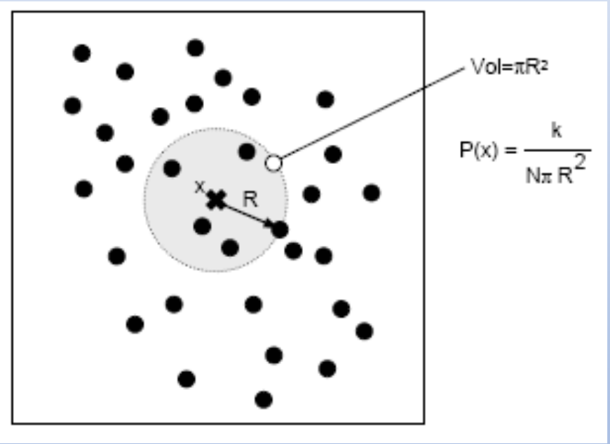
In this 2-D example, a circle centred at grows until its radius reaches the -th nearest sample. Its volume is , so (the figure writes for , and for the density estimate ).
Step 3: what the estimate looks like
Two kNN estimates of a 1-D density from eight points, for and :
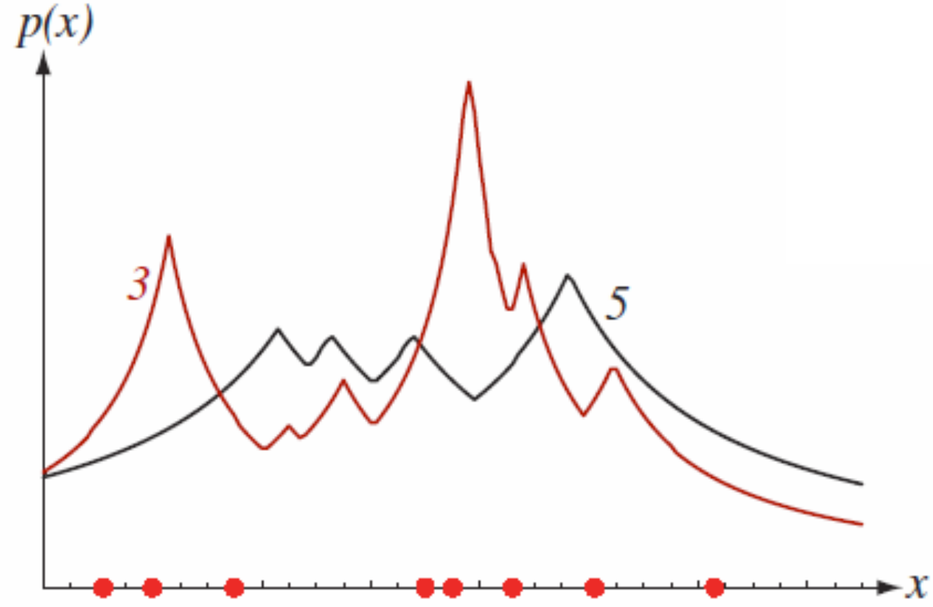
Reading the figure:
- the estimate is high where the samples are close together, because a small already holds samples there
- gives a smoother estimate than , because each estimate uses more samples
- the estimates have sharp corners (jumps in the slope), and these generally lie away from the sample positions, where the -th nearest sample switches from one sample to another
- far from the samples, keeps growing, so in 1-D the estimate falls only like and never reaches zero
What follows:
- the region adapts to the data by itself: small in crowded areas and large in empty ones
- because the tails fall so slowly, the area under the estimate is in fact infinite (the area under grows without limit), so it is not a true PDF, only a local density estimate
Why do we need this
It avoids choosing one cell size for the whole space. It also leads to a classifier: grow one region around over the samples of all classes together, and the decision becomes a vote among the samples inside it.
Next step
kNN Classifier turns the nearest samples into a decision.
Visual 1: fixed volume against fixed count
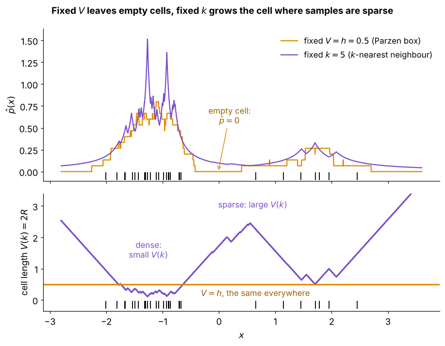
Same samples, with a dense group on the left and a few spread out on the right:
- top: the box with fixed gives in the gap where its cell holds no sample, while always gives a positive value
- bottom: the cell length that just holds samples, small inside the dense group and large in the gaps
- so kNN uses a small region where the data allow it and a big one only where it must, which is Step 2 of this note
- the sharp corners of the purple curve sit where the -th nearest sample switches from one sample to another
Visual 2: tails that never die
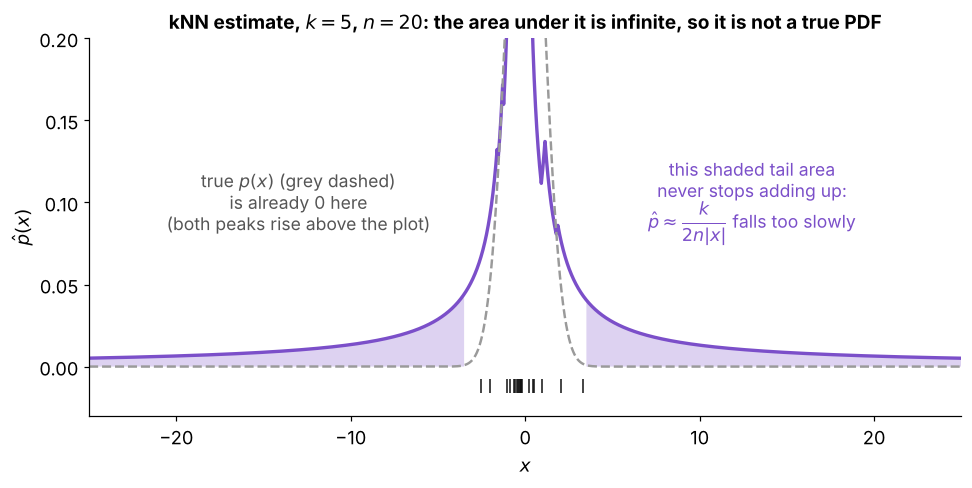
How to read it:
- far from the samples the -th nearest sample is about away, so and
- the true PDF (grey dashed) is already zero there, but the purple tails are still above zero
- the shaded tail area keeps adding up the further out you go, like the area under , so the total area is infinite
- so the kNN estimate is a local density value and not a true PDF, as Step 3 says