Introduction
The -nearest neighbour (kNN) classifier classifies by a majority vote among its nearest training samples. It uses the same growing region as kNN estimation, with the samples of all classes mixed together. With it is the nearest-neighbour (NN) classifier.
Main idea
Find the $k$ training samples closest to $\mathbf{x}$ and choose the class with the most samples among them. The NN boundary is made of flat pieces between samples of different classes, straight line segments in 2-D. With a very large number of training samples, the NN error rate is at most about twice the Bayes error, and the kNN error rate moves closer to the Bayes error as $k$ grows.
Overview
The classifier needs no training step, only the stored samples:
Step 1: kNN rule
The kNN rule is a generalization of the NN rule. Given a set of training samples and a test point :
- find the training points closest to , called
- collect their labels (here is a class label, unrelated to the parameter vector of the ML notes)
- classify to the class with the greatest number of representatives in
In other words, the classification is a majority vote among the nearest neighbours of .
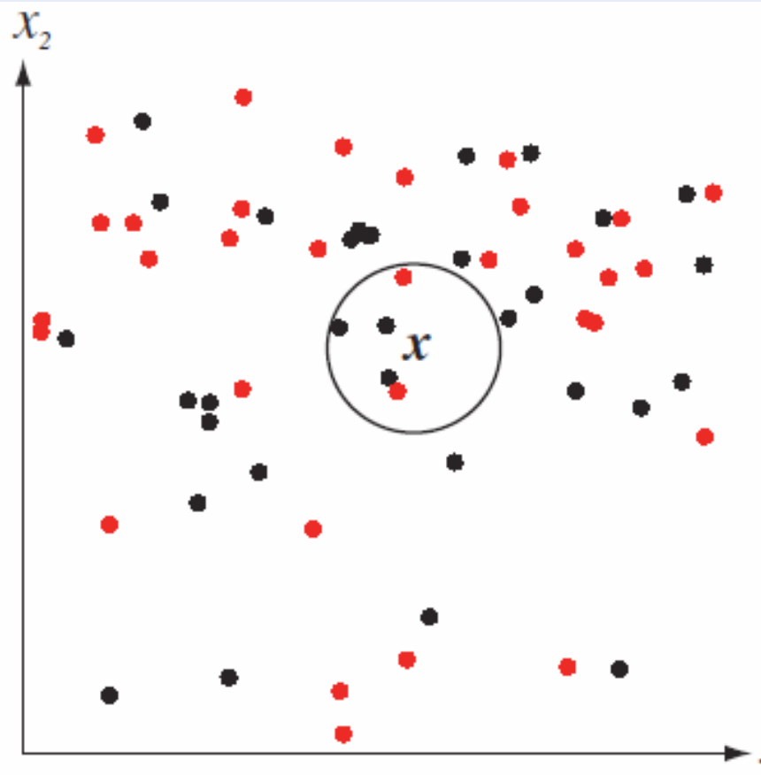
The query starts at the test point and grows a spherical region until it encloses training samples. In this case, the circle holds 3 black and 2 red samples, so is labelled as the black class.
Step 2: why a vote
The vote comes from the MAP rule. The key is that the region is grown once, over the samples of all classes pooled together, and every class is then counted inside that same region. Estimating each class density with its own separate kNN region would not give a vote.
A way to check this yourself:
- grow one region of volume around over the samples of all classes pooled together, so it holds samples in total, with of them from class , which has of the training samples
- is then the same for every class, and only the count changes from class to class
- write with , and , as in Nonparametric PDF Estimation, and with and
- put them into and see which letters are the same for every class
- recall that the MAP rule has the smallest error, so a rule that always picks the MAP class also has the smallest error
Step 3: nearest-neighbour rule
Let be a set of labelled prototypes (training samples), and let be the prototype nearest to . The nearest-neighbour (NN) rule assigns the label of .
More formally, for labelled training samples , where each label is one of :
How to read it:
- is the Euclidean distance from to sample
- here is the index of the nearest sample, and not a count
- , the decision, is the label of that nearest sample
This is also called the 1st-nearest-neighbour classifier, the kNN rule with .
Step 4: decision boundary
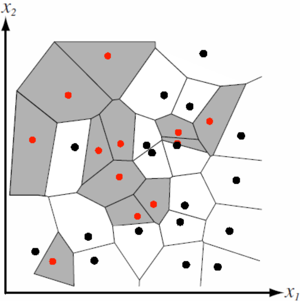
What the figure shows:
- the NN classifier splits the space into cells, one cell for each training sample
- each cell holds the points that are closer to its sample than to any other sample (a Voronoi tessellation)
- the edge between two neighbouring cells is the perpendicular bisector of the two samples, the set of points equally far from both
- the NN rule is the minimum distance classifier with every training sample as its own template, and like it, it uses the Euclidean distance, which ignores the shape of each class cloud
- the grey cells belong to the red class and the white cells to the black class
- the decision boundary is made of the cell edges between samples of different classes, so it is piecewise linear and can be very complex
Step 5: NN error rate
For a very large number of training samples, the error rate of the NN classifier is bounded by:
where is the error rate of the NN classifier, is the Bayes error (the error rate of the MAP rule, the smallest possible) and is the number of classes.
How to read the two bounds:
- the lower bound says no classifier beats the Bayes classifier, the NN classifier included
- in the upper bound, the term is small when is small, so the bound is just under
- so with enough samples, the NN error is at most about twice the Bayes error, using no model and no training
Why about twice, for two classes:
- at a given , the true class is itself random: it is with probability
- with very many samples, the nearest sample lies almost at , so its label is an independent draw from the same posteriors
- let , the Bayes error at , since the MAP rule is wrong exactly when the true class is the less likely one
- the two labels disagree with probability , which is just under when is small
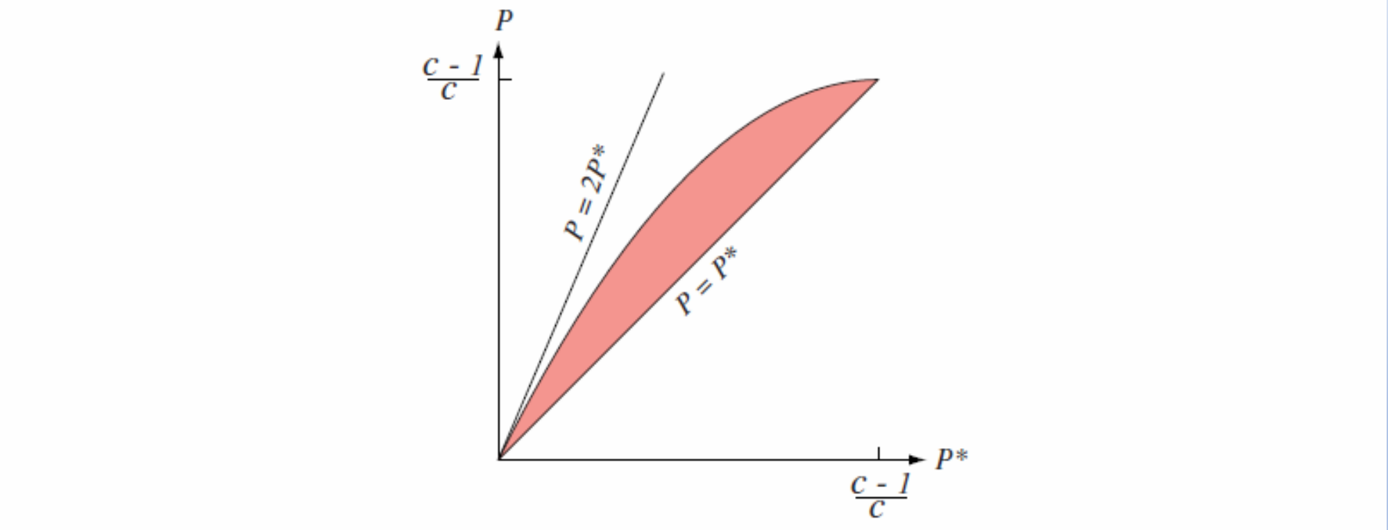
Reading the figure:
- the shaded region between the line and the upper curve is where the NN error rate can lie
- the upper curve stays below the line , and touches it only near
- both axes end at , the error of a blind guess among equally likely classes, where the two bounds meet
Step 6: kNN error rate
For the kNN rule in a two-class problem:
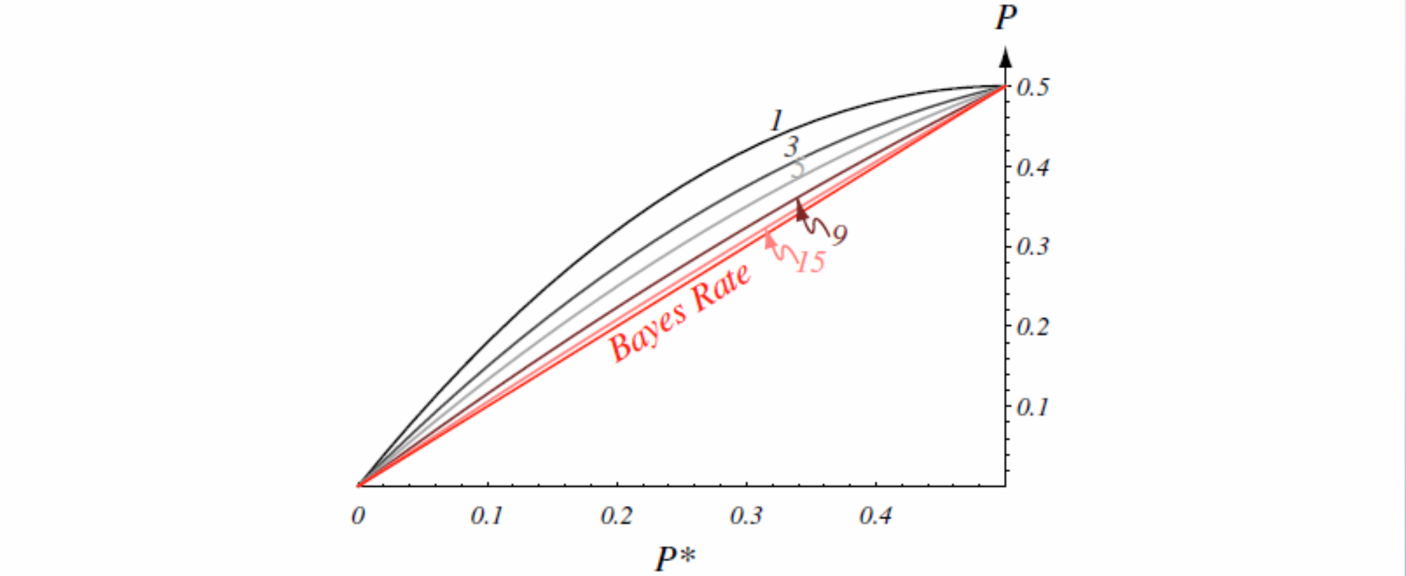
Reading the figure:
- the top curve, , is the NN upper bound of Step 5 with , , which is why the axes end at
- each curve is the upper bound of the kNN error rate for one value of , and is odd so that a two-class vote can never tie
- a larger moves the error rate closer to the Bayes rate , because the share of each class among more neighbours behaves like a better estimate of its posterior (Step 2 lets you check why)
- when , the estimated probabilities match the true probabilities, and the error rate equals the Bayes rate,
- this needs the number of samples to grow much faster than , so that all neighbours are still close to
Why do we need this
It is the simplest classifier that needs no model: store the samples and vote. Its error bounds show how close counting alone can get to the best possible decision.
Next step
Nonparametric estimates can be far from the true PDF when samples are few. Maximum Likelihood Estimation instead assumes a model with a few parameters and fits them.
Visual 1: boundary as grows
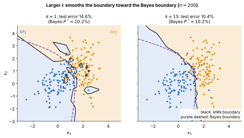
Two Gaussian classes with 100 training samples each; the purple dashed curve is the Bayes boundary computed from the true PDFs:
- left, : the boundary bends around single samples and makes islands, so the test error is 14.6% against the Bayes error 10.2%
- right, : the vote averages over more neighbours, the boundary is smoother and close to the Bayes boundary, and the test error is 10.4%
- this matches Steps 5 and 6: NN is within about , and a larger moves the error toward
Visual 2: vote equals MAP
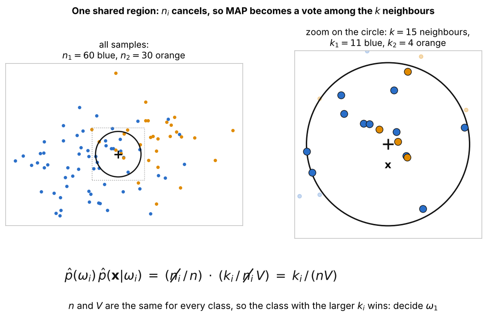
A check of Step 2 with unequal classes, and :
- left: one circle around , grown over the samples of both classes together until it holds
- right, zoomed: count them yourself, blue and orange
- below: times , and the on top and bottom cancel, leaving
- and are the same for both classes, so MAP picks the class with the larger ; the prior is not lost, a bigger class simply has more samples near