Introduction
Maximum likelihood (ML) estimation is a parametric method. It assumes the PDF has a known form with an unknown parameter vector , and picks the that makes the observed training samples most probable. Here the bar means "with the parameters set to ": is a fixed unknown, not a random variable or a class.
Main idea
The samples are independent, so the probability of all of them is the product $p(D|\boldsymbol{\theta})=\prod_k p(\mathbf{x}_k|\boldsymbol{\theta})$, called the likelihood. Choose $\hat{\boldsymbol{\theta}}=\arg\max_{\boldsymbol{\theta}}\sum_{k=1}^{n}\ln p(\mathbf{x}_k|\boldsymbol{\theta})$, and find it by solving $\nabla_{\boldsymbol{\theta}}\ln p(D|\boldsymbol{\theta})=\mathbf{0}$.
Overview
The method is a chain of four moves:
Step 1: why a parametric model
A PDF learned from training samples by a nonparametric method can deviate greatly from the true PDF of the population, especially when there are only a few training samples.
If general knowledge about the problem lets us model the conditional PDF, that is, write it as a mathematical function with unknown parameters, this problem becomes much less severe. Parameterizing the conditional PDF is called the parametric method.
What this means:
- neural networks and deep learning are also parametric methods, with very many parameters
- the simplest case is a Gaussian with mean and covariance matrix , the matrix of the variances of the features and the covariances between them (Gaussian Discriminant Function explains both)
- and are unknown, but the problem shrinks from estimating a whole unknown function to estimating only the parameters and
Step 2: idea from an example
We use a set of training samples , drawn independently from the density , to estimate the unknown parameter vector .
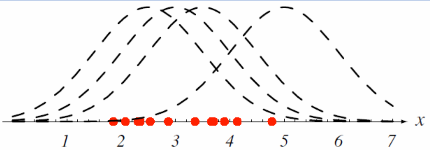
Reading the figure:
- the red points are 1-D training samples, known or assumed to come from a Gaussian of a known variance but an unknown mean
- the dashed lines are four candidate PDFs, the same Gaussian shape at four different means
- the question is which candidate to choose
The natural answer: choose the PDF under which the samples we actually observed are most probable, which is the curve centred among the samples. A curve centred among the samples gives each sample a high density. A curve far to one side gives many samples a density near zero, so it explains the data badly.
Step 3: likelihood
Turn that idea into a formula:
- the probability (density) that one sample occurs is
- all training samples are collected independently, so the probability that all of them occur is the product of the single probabilities
With the data fixed, is a function of only, called the likelihood of with respect to the set of samples . Select the parameter so that best supports the observed samples, that is, so that the likelihood is maximal:
This method is called maximum likelihood (ML) estimation.
Step 4: log-likelihood
An analytical solution of the product is often hard to get:
- it multiplies many functions of , and the derivative of a long product is messy
- each is often a nonlinear function of , such as an exponential
Taking the logarithm fixes both:
- is monotonically increasing, so the that maximizes also maximizes
- turns a product into a sum,
- undoes an exponential, , which simplifies Gaussian-type PDFs
So maximize the log-likelihood instead:
Step 5: set the gradient to zero
The solution is found with standard differential calculus: at a maximum, the gradient is zero. A zero gradient can also mark a minimum or a saddle point, so check that the solution is a maximum. For the Gaussian in the next note it is. The derivative of a sum is the sum of the derivatives, so:
If there are parameters to estimate, is a -component vector. The gradient is the vector of partial derivatives against all components of :
So "gradient equals zero" is equations, one per parameter, and solving them together gives the estimates.
Why do we need this
It is the standard recipe to fit any model to data: write the log-likelihood, take its gradient, set it to zero. With a good model, a few parameters estimated from few samples beat a whole PDF estimated by counting.
Next step
Gaussian ML Estimates applies this recipe to a Gaussian.
Visual 1: why the log keeps the peak
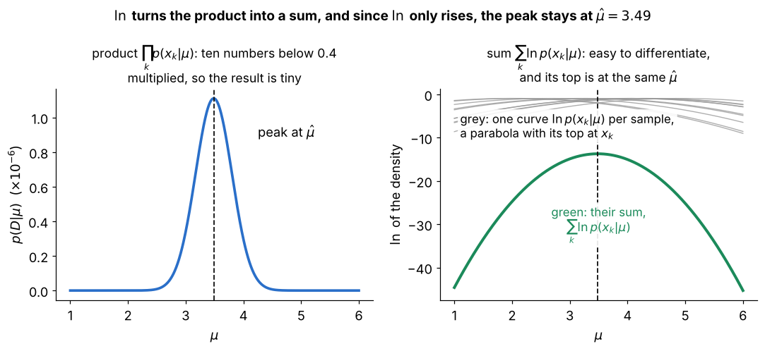
Ten samples from a Gaussian with known, as functions of the candidate mean :
- left: the likelihood multiplies ten densities, each below , so the product is tiny (about ) and awkward to differentiate
- right, grey: turns each factor into its own term , a simple parabola with its top at that sample
- right, green: the log-likelihood is just the sum of these parabolas, so the product has become a sum, as in Step 4
- only rises, so the highest point stays the highest point: both curves peak at the same , the sample mean
Visual 2: zero gradient as balanced pulls
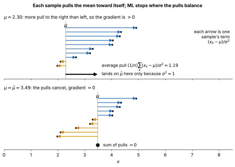
For a Gaussian mean, the gradient term of one sample is , drawn as an arrow from toward the sample:
- top, : more samples sit to the right, so the pulls add to a positive gradient and the log-likelihood rises if moves right
- the average pull lands exactly on here only because ; in general it only points the right way
- bottom, : the left and right pulls cancel, so , which is Step 5