Introduction
The Parzen-window approach fixes the size of the region around and counts the samples inside it with a kernel function. Once the count is written as a sum of kernels, the box kernel can be swapped for any smooth PDF. It interpolates the discrete training samples into a continuous PDF.
Main idea
$\hat{p}(\mathbf{x})=\frac{1}{nh^d}\sum_{i=1}^{n}K\left(\frac{\mathbf{x}-\mathbf{x}_i}{h}\right)$: put one kernel of width $h$ on every training sample and average them. Any PDF can be the kernel $K$, and the result is then a valid PDF. The width $h$ controls how smooth the estimate is.
Overview
Every training sample contributes one bump, and the estimate is their average:
Steps 1 and 2 get this formula from counting in a box. Step 3 shows any PDF can be the bump. Steps 4 and 5 show what the width does.
Step 1: count with a function
In Nonparametric PDF Estimation, a sample is inside the hypercube of side around if for all . Write this test as a function, called the Parzen window:
The names Parzen window, box kernel and rectangular kernel all mean this . From Step 3 on, "kernel" means any , and the box is one choice.
Then the number of samples inside the cell is a sum:
How to read it:
- is the offset of sample from , measured in units of
- exactly when is inside the cell, and otherwise
- adding over all samples counts the samples inside the cell
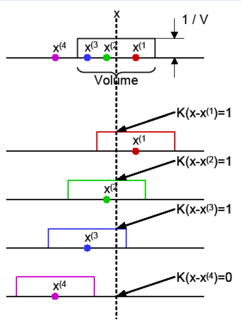
Reading the figure:
- the top line shows the cell of width (the volume) centred at , with height
- each lower line shows one box kernel, centred at one sample
- the boxes of , and cover , so each gives
- the box of does not cover , so it gives
- the box is symmetric, so "the cell at contains " and "the box at covers " are the same test
- the figure writes for and leaves out the , and it draws each box with height so that the boxes covering add up to directly
Step 2: density estimate
Put the count into with :
Using the box window on 1-D data
Points to settle before counting:
- the window size is the side length , and in 1-D the volume is
- sample counts at when
- a sample exactly away sits on the edge of the window, so decide whether it counts, and state your choice
- a point with no sample inside its window gets , which the box kernel allows
Step 3: general kernel
The rectangular kernel gives an unsmoothed PDF: the box jumps from 0 to 1 at its edges, so the estimate jumps too. In fact any function can be the kernel as long as:
These are exactly the two conditions for to be a PDF. The box kernel of Step 1 already meets both: it is never negative, and it equals 1 on a unit cube of volume 1 and 0 everywhere else, so its integral is 1. A smooth kernel keeps these two properties and removes the jumps.
With a smooth kernel, nothing is counted as in or out any more: each sample adds a weight that falls off with its distance from , so near samples count a lot and far samples count a little. The two conditions make each term of the estimate integrate to 1:
Why, by a change of variable:
- let , so each of the components is divided by
- then , one factor per dimension
- so the integral above is
What follows:
- each term is itself a PDF, centred at
- is the average of PDFs, so it is never negative and integrates to , which makes it a valid PDF
- so any PDF can serve as the kernel function
This is the Parzen-window approach. It interpolates the discrete points into a continuous PDF .
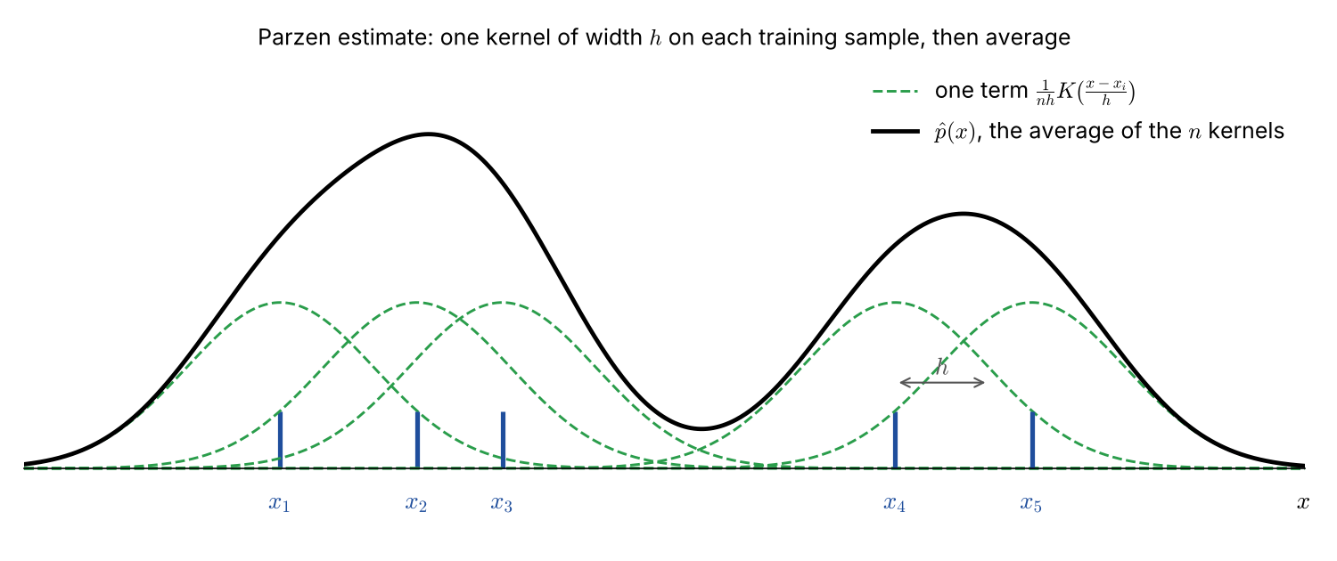
The training samples are single points (blue). Each gets one kernel of width (green, dashed), scaled by . Their sum (black) is the continuous estimate.
Link to sampling
Sampling turns a continuous signal into discrete points, and reconstruction gets a continuous signal back by placing an interpolation kernel on every sample and adding them up. To compare this with the Parzen window, match the parts:
- what plays the role of the discrete samples
- what plays the role of the interpolation kernel
- what the width does, compared with the width of the interpolation kernel
- where the information sits: in the sample values, or in the sample positions
Step 4: Gaussian kernel
A common smooth kernel is the standard Gaussian:
What it becomes inside the estimate:
- is the multivariate Gaussian with mean and covariance (Gaussian Discriminant Function explains the general formula): a round bell over dimensions, with the squared length of
- with , the term is a Gaussian centred at with standard deviation in every dimension
- in 1-D it is , the usual Gaussian with mean and standard deviation
- so is the width of every bump
A 1-D example, with the number of samples in the rows and the starting width in the columns:
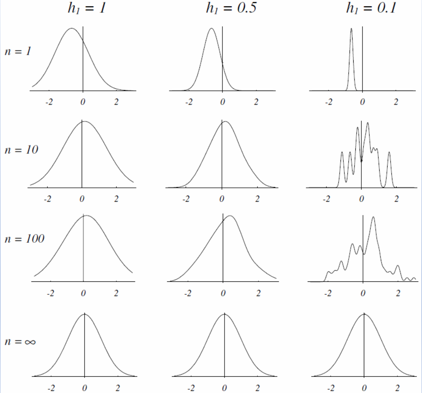
Reading the figure:
- with , the estimate is just one Gaussian kernel centred at the sample
- a small with few samples gives a spiky, noisy estimate, one spike per sample
- a large gives a smooth estimate, but it can hide detail
- is the width used when , and the width shrinks as grows, in this figure
- so as the bumps get narrower but there are many more of them, and every column reaches the true PDF
- if stayed fixed, the estimate would stay a blurred copy of the true PDF, even with infinite samples
Choosing : there is no single best value. It must shrink as grows, as in , which is the small-region need of Nonparametric PDF Estimation, while staying wide enough that each bump still overlaps its neighbours.
Step 5: 2-D examples
A single 2-D training sample with a Gaussian kernel of width :
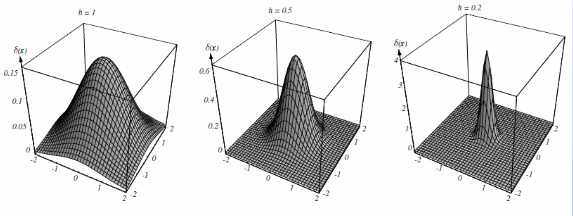
A smaller gives a narrower and taller peak. The vertical axis is the kernel term , not a delta function, and its peak is . The volume under each kernel stays 1, so the vertical scales are different.
Five 2-D training samples with the same three widths:
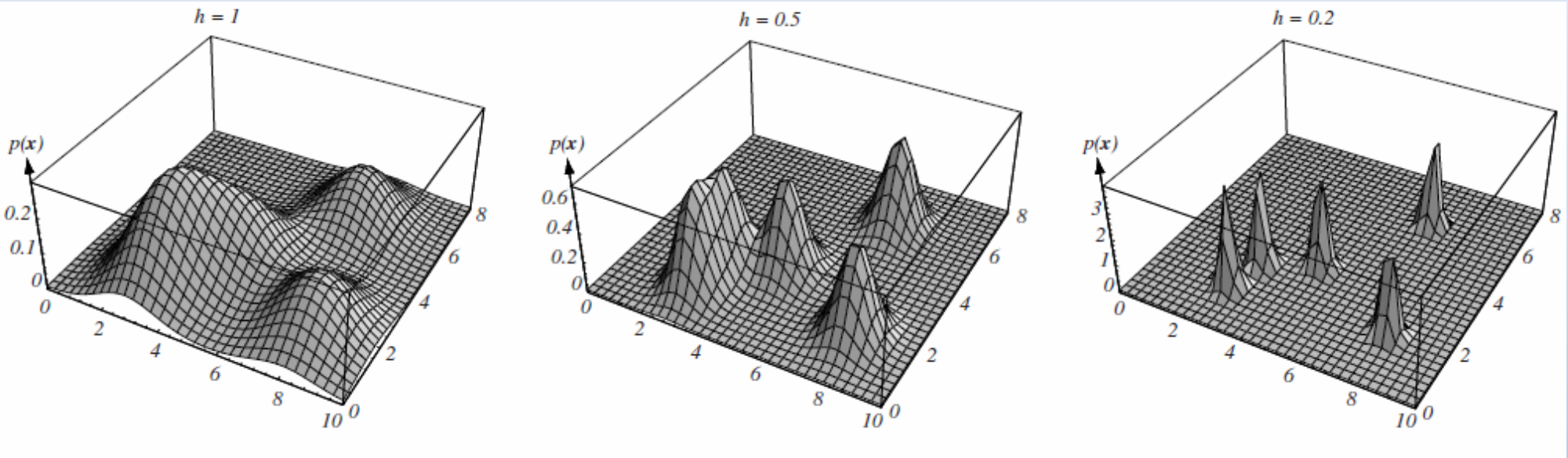
What changes with :
- merges the five kernels into one smooth surface
- shows separate bumps
- gives five sharp spikes, one at each sample
Step 6: link to neural networks
Probabilistic neural networks and RBF neural networks are almost equivalent to the Parzen-window approach: they place bump-shaped units on stored samples (or on centres learned from them) and add up the outputs.
Why do we need this
It turns a handful of points into a smooth PDF that can be evaluated at any , with one setting, the width , to trade detail against noise.
Next step
k-Nearest Neighbour Estimation fixes the number of samples instead of the cell size.
Visual 1: box kernel against smooth kernel
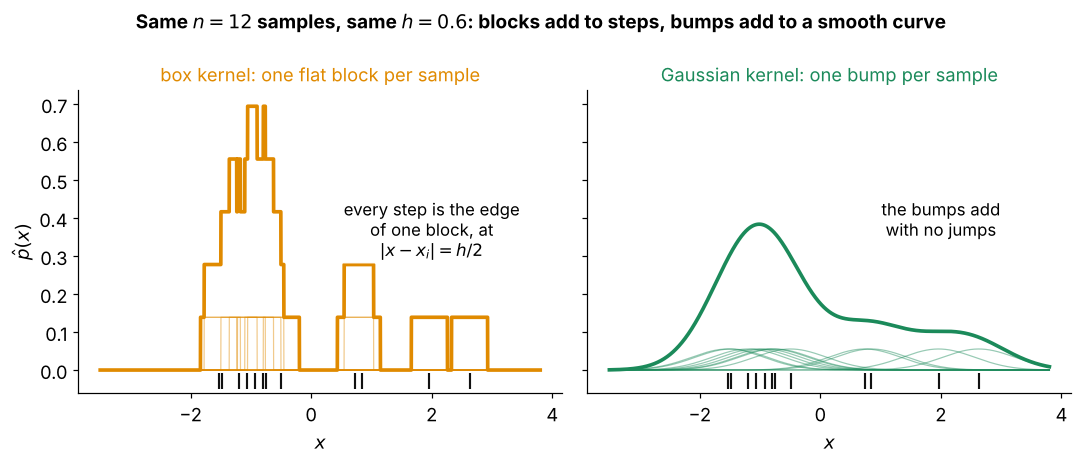
Both panels use the same samples and the same width , so only the kernel shape changes:
- the faint lines are the single kernel terms , one per sample
- left, the box kernel of Step 1: each sample adds a flat block, so the sum is a staircase with a step at every block edge
- right, the Gaussian kernel of Step 4: each sample adds a smooth bump, so the sum has no jumps
- both sums are averages of PDFs, so both are valid PDFs, as Step 3 shows
Visual 2: why the factor
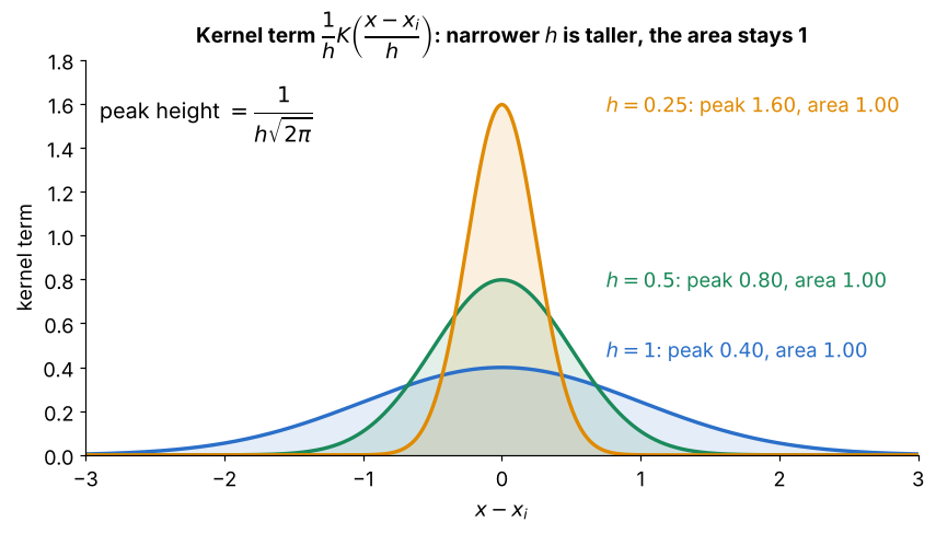
One kernel term in 1-D with a Gaussian :
- halving makes the bump half as wide and twice as tall, with peak
- the area stays for every , which is the change of variable in Step 3
- without the factor a narrow kernel would hold less area, and would no longer integrate to 1