Introduction
The Mahalanobis distance measures how far a point is from a class mean in units of that class's own spread. It is the distance a Gaussian classifier really uses: a point is "close" to a class when it is within a few spreads of the mean, in whichever direction it lies. The definitions and the 1-D and 2-D cases are in Mahalanobis and Euclidean Distance.
Main idea
$d_{\Sigma}(\mathbf{x},\boldsymbol{\mu})=(\mathbf{x}-\boldsymbol{\mu})^T\boldsymbol{\Sigma}^{-1}(\mathbf{x}-\boldsymbol{\mu})=\sum_k\frac{y_k^2}{\lambda_k}$, where $y_k$ is the offset along eigenvector $k$ and $\lambda_k$ the spread there. Each part of the offset is divided by the spread in its own direction, so a step along a thin axis of the cloud counts much more than the same step along a wide axis. Points with equal Mahalanobis distance lie on an ellipse shaped like the cloud, and these are the points of equal Gaussian density.
What it is
How to read it:
- these notes use the squared form, without a square root
- with it is the squared Euclidean distance
- in 1-D it is , the square of "how many standard deviations away"
Physical meaning
Write the offset in the eigenvector axes of , . Then:
What this says:
- a ruler that stretches with the cloud: along each axis of the cloud, the offset is measured in units of the spread along that axis
- thin directions count more: an offset along an axis with small is divided by a small number, so it counts a lot, because the class rarely goes that far in that direction
- wide directions count less: an offset along an axis with large is ordinary for this class, so it counts little
- contours are ellipses: the points with the same form an ellipse with the same axes as the cloud
- ordinary distance after whitening: squash the cloud into a round ball with unit spread, and is the plain squared Euclidean distance there (Inverse Covariance and Whitening in Pattern Recognition)
- link to probability: the Gaussian density of one class is proportional to , so within one class a smaller Mahalanobis distance always means a higher likelihood
When it equals the Euclidean distance up to a scale:
- with , , so the nearest mean is the same with either distance
Where it is used
| Note, step | What the Mahalanobis distance does there |
|---|---|
| Gaussian Discriminant Function, Step 4 | is times the Mahalanobis distance to class , plus a bias from the prior and |
| Quadratic Classifier | each class measures distance with its own , so the boundaries curve |
| Linear Classifier | all classes share one , so they use the same ruler and the boundaries are flat |
| Minimum Distance Classifier | with and equal priors, it reduces to "nearest mean in Euclidean distance" |
| Discriminant Function in Eigenspace, Step 5 | the distance is written as in the class's eigenvector axes |
| Discriminant Function in Eigenspace, Step 6 | a training that is too small makes too large, so the distance is dominated by unreliable directions |
| Eigenvalue Regularization, PCA for Classification | the fixes change the weights in this sum: raise the small , or drop their terms |
| kNN Classifier, Parzen Window | these use the plain Euclidean distance, which ignores the shape of each class cloud |
| Attention as Weighted Sum of Values, Step 1 | the score has the same form, a vector times a matrix times a vector, with the middle matrix learned instead of |
Common traps
Points that are easy to get wrong:
- the squared form and the square-root form give the same nearest mean, but the formulas in these notes use the squared form
- the Mahalanobis distance needs , so it breaks when is singular (a zero eigenvalue)
- a smaller Mahalanobis distance alone does not decide the class: the Gaussian classifier also adds the bias with the prior and
Test yourself
Two points are the same Euclidean distance from the mean. Why can their Mahalanobis distances differ?
One may lie along a wide axis of the cloud and the other along a thin axis. The thin-axis offset is divided by a smaller spread, so it is much farther in Mahalanobis distance.
Why is the Mahalanobis distance the "right" distance for a Gaussian class?
The Gaussian density of one class depends on only through , so within one class, comparing Mahalanobis distances is comparing likelihoods. Between classes with different , the term also counts.
Why does the small-sample problem show up in the Mahalanobis distance?
The distance divides by every . The smallest training eigenvalues are too small, so their terms blow up for a new sample, even if that sample truly belongs to the class.
Why do we need this
The Mahalanobis distance is the bridge between the covariance matrix and the classifier. It explains why the Gaussian classifiers have the boundaries they have, and it is exactly where the unreliable small eigenvalues do their damage.
Visual 1: Mahalanobis is ruler distance after whitening
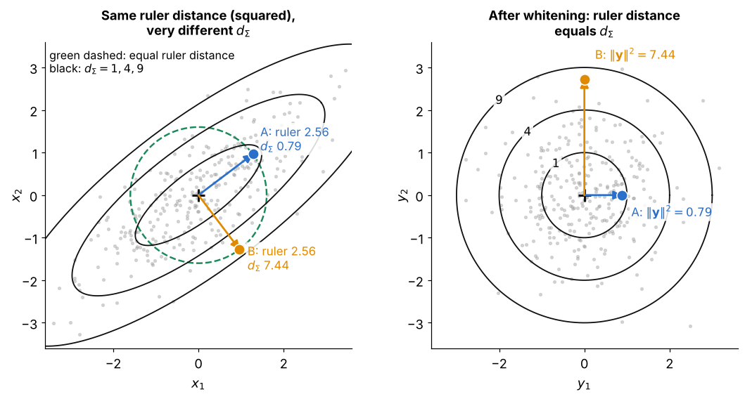
A lies on the wide axis and B on the thin axis, both on the dashed circle:
- left: both lie on the green circle, so their squared ruler distances are equal (), but A is inside and B is outside
- gives for A and for B, because B goes far in a direction the class rarely goes
- right: after whitening the black ellipses become circles, and the plain gives exactly the same two numbers
- so the contours of equal are ellipses shaped like the cloud, the points of equal Gaussian density
Visual 2: each axis adds its own term
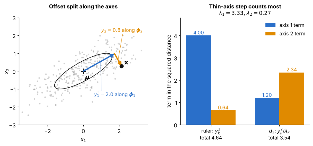
This is for one point:
- left: the offset is split into along the wide axis and along the thin axis
- Euclidean: the wide-axis term is most of the total
- Mahalanobis: dividing by and flips this, and the shorter thin-axis step gives the larger term ( against )
- a too small training makes its term blow up in the same way, which is where the small-sample problem shows up