Introduction
The nonparametric approach estimates a PDF directly from the training samples, without any assumption about the form of the model. The idea is to count how many samples land near : where samples are crowded, the density is high.
Main idea
The probability of a small region around $\mathbf{x}$ is about $p(\mathbf{x})V$, and the fraction of training samples inside it is about $\frac{k}{n}$. Setting the two equal gives $\hat{p}(\mathbf{x})=\frac{k}{nV}$. A different shape or size of the region gives a different estimate.
Overview
The whole estimate is one fraction:
A density is probability per unit volume, so it is "how much of the data is here" divided by "how big here is".
Step 1: probability of a region
By the definition of a PDF, the probability that a random sample from falls in a region centred at is the integral of the PDF over that region, where runs over the points of the region:
where is the volume of the region .
Why the approximation holds:
- if the region is small, hardly changes inside it, so for every in the region
- the constant then comes out of the integral, leaving , because integrating 1 over a region gives its volume (its length in 1-D, its area in 2-D)
Step 2: count the samples
If of all training samples of this class fall in the region, the estimate of is:
Why this works:
- each sample lands in the region with probability , independently of the others
- so out of samples, about land in the region
- the observed count therefore gives , the fraction of samples that landed there
Step 3: combine
Set the two expressions for equal, , and divide by :
This is called the nonparametric approach because it makes no assumption about the form of .
Step 4: procedure
To estimate from training samples:
- for a given value of , select a region (cell) of volume centred at
- count the number of training samples inside the cell
- estimate
- repeat for every value of where the PDF is needed
Different shapes and sizes of the cell give different estimates of the PDF.
Why the size matters:
- Step 1 needs a small region, so that is nearly constant inside it
- Step 2 needs many samples inside the region, so that is a reliable fraction
- with a fixed number of samples, a smaller region holds fewer samples, so the two needs pull against each other
- more samples let the region shrink while still holding enough of them, and the next two notes handle the trade-off in two ways: fix (Parzen window) or fix (-nearest neighbour)
Step 5: hypercube region
In general has dimensions. Choose as the region a -dimensional hypercube of side length centred at , so its volume is . A sample falls inside the hypercube if:
How to read it:
- along each dimension , the cube reaches to each side of
- says the sample is within that reach along dimension
- the sample is inside the cube only if this holds along every dimension
- in 1-D the cube is an interval of length , so
Step 6: two ways to choose the region
In , one of and is fixed and the other is read from the samples:
| Fixed | Found from the samples | Estimate | Method |
|---|---|---|---|
| volume | number of samples | Parzen window | |
| number of samples | volume | -nearest neighbour |
Why do we need this
It is the simplest way to get a PDF from data with no assumptions at all. Both the Parzen window and the -nearest neighbour method are this one formula with a different choice of what to fix.
Next step
Parzen Window fixes the cell size, writes the count as a sum, and turns the box into any smooth kernel.
Visual 1: count in a cell
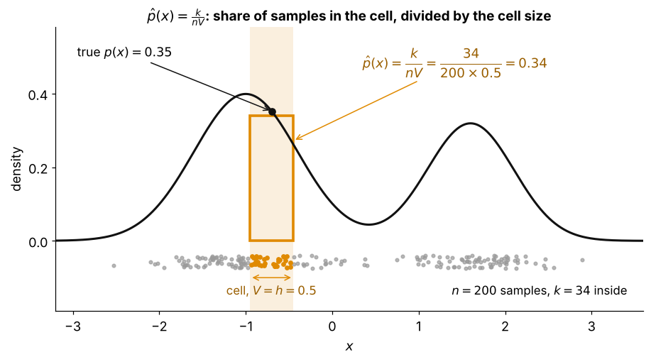
How to read it:
- the black curve is the true , and the dots below are training samples
- the shaded cell has width around , so in 1-D , and the orange samples are the inside it
- the orange box has height and area , the share of samples in the cell
- its height is close to the true value , which is Steps 1 to 3 of this note in one picture
Visual 2: small cell against large cell
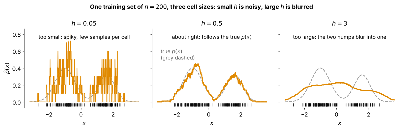
One training set, with worked out at every for three cell sizes:
- small : each cell holds only a few samples, so jumps between 0, 1 and 2 and the estimate is a row of spikes
- middle : the cell is small enough that is nearly constant inside it and big enough to hold many samples, so the estimate follows the true curve
- large : changes a lot inside one cell, so the two humps are averaged together into one flat bump
- this is the pull between the two needs in Step 4, and more samples move the good to a smaller value