Introduction
A neural network learns the mapping from input to output directly from training pairs, without first estimating probability densities. This topic builds the traditional network, the multilayer perceptron (MLP), from a single neuron up, then shows how it is trained and what can still go wrong.
Main idea
A neuron computes a weighted sum of its inputs and passes it through an activation function. Stacking neurons in layers gives an MLP, $\mathbf{y}=f\left(\mathbf{V}^Tf(\mathbf{W}^T\mathbf{x})\right)$, and the activation must be nonlinear or the layers collapse into one. Training means minimizing the squared error between outputs and targets: one linear layer has a closed-form least squares answer, gradient descent reaches it step by step, and backpropagation extends gradient descent to the hidden layers. Even then, training can stop in a local minimum, and a perfect fit to the training data can generalize badly.
Overview
The topic has three parts, each building on the one before:
What each part covers:
- network architecture and neuron model: what one neuron computes, which activation functions are used, and how neurons connect into an MLP
- optimization and iterative (error correction) learning: the best weights of one linear layer, found in closed form by least squares or step by step by gradient descent
- MLP and the backpropagation learning algorithm: how gradient descent reaches the hidden layers, and why a trained network can still fail
Where this fits
The Bayes classifiers needed , the probability density of within class , before they could decide which class belongs to. A neural network skips that step: it adjusts its weights until its outputs match the targets on the training data. In the computer vision system it can do the classification stage, and deeper networks also take over feature extraction.
Notation
These notes use the letters below:
| Symbol | Meaning |
|---|---|
| input vector, inputs | |
| outputs of the hidden layer, hidden neurons | |
| network outputs, output neurons | |
| target (desired) outputs | |
| first-layer weights, (one more row if the bias is included), where joins input to hidden neuron | |
| second-layer weights, (one more row if the bias is included), where joins hidden neuron to output | |
| activation function | |
| error to minimize | |
| learning rate | |
| number of training samples, in Least Squares Single Layer Network |
Some letters change meaning, so watch for these:
- is the number of hidden neurons here, not the dimension of as in earlier notes
- the weighted sum of a neuron is called and in Neuron Model, in Activation Functions, and (hidden) or (output) in Backpropagation
- and as weighted sums are unrelated to the second-layer weights and , used from Multilayer Perceptron Structure on
- alone is a number of samples, while and are weighted sums
- is the number of inputs, except in the training procedure of Backpropagation and in the learning curve figures, where it counts training samples
- numbers the inputs in and , but numbers the training samples in , and in the least squares and LMS notes
- bold is the target of one sample, except in Least Squares Single Layer Network, where it is the row of the targets of all samples
Targets and classes
For classification, each class label is coded as a target number, and each output is read back as a class:
- with one output and two classes, use the target for one class and for the other, and read the class from the sign of the output
- with classes, use outputs, with target 1 at the output of the true class and 0 (or ) at the others, and pick the class whose output is largest
- why the largest output: with squared error and these 1-of- targets, the outputs of a well-trained network approach the posteriors , so picking the largest output is the MAP rule of the Bayes classifiers
- "two-layer network" counts the layers of neurons that compute, so the input layer is not counted, and a "single layer network" has no hidden layer
Reading order
The notes follow one line of thought, each step using the one before:
- Neuron Model: what does one artificial neuron compute, and how does the threshold become a weight?
- Activation Functions: which functions turn the weighted sum into the output, and how do they differ?
- Multilayer Perceptron Structure: how do neurons stack into layers, how many weights are there, and why must the activation be nonlinear?
- Least Squares Single Layer Network: what are the best weights of a one-layer linear network, in closed form?
- LMS Gradient Descent Learning: how can the network reach those weights one sample at a time?
- Backpropagation: what can two layers represent, and how are the hidden weights trained?
- Local Minima and Overfitting: why can training still fail, even when the training error is small?
Concept map
flowchart TD
    A["Neuron model<br/>y = f(wᵀx), threshold as weight w₀"] --> B["Activation functions<br/>step, piecewise linear, sigmoid, ReLU"]
    B --> C["Multilayer perceptron<br/>y = f(Vᵀ f(Wᵀx))<br/>linear f collapses to one layer"]
    C --> D["Single layer least squares<br/>w = (XXᵀ)⁻¹Xtᵀ"]
    D --> E["LMS gradient descent<br/>w ⇐ w + η(t − y)x"]
    E --> F["Backpropagation<br/>chain rule through the layers"]
    F --> G["Local minima and overfitting"]
Why do we need this
Real classes are rarely Gaussian, and their densities are hard to estimate in high dimensions. A neural network learns the decision directly from examples, and with enough hidden neurons it can draw any boundary. The same building blocks lead to CNNs and Transformers.
Key math ideas
The math ideas this topic relies on, and where each one appears:
- Dot product and projection: the weighted sum in the Neuron Model, and the update that moves the template toward or away from a sample in LMS Gradient Descent Learning
- Gradient: the downhill step in LMS Gradient Descent Learning and Backpropagation, the closed-form solve in Least Squares Single Layer Network, the slope of the activation in Activation Functions, and the trap in Local Minima and Overfitting
- Inverse covariance and whitening: undoes the spread of the inputs, in Least Squares Single Layer Network
- Rank: is singular with fewer samples than inputs, in Least Squares Single Layer Network
- Likelihood: squared error is maximum likelihood under Gaussian noise in Least Squares Single Layer Network, and overfitting is ML hugging its data in Local Minima and Overfitting
- Softmax and posterior: with 1-of- targets the outputs approach the posteriors, so the largest output is the MAP class
Visual 1: what the MLP adds over one linear layer
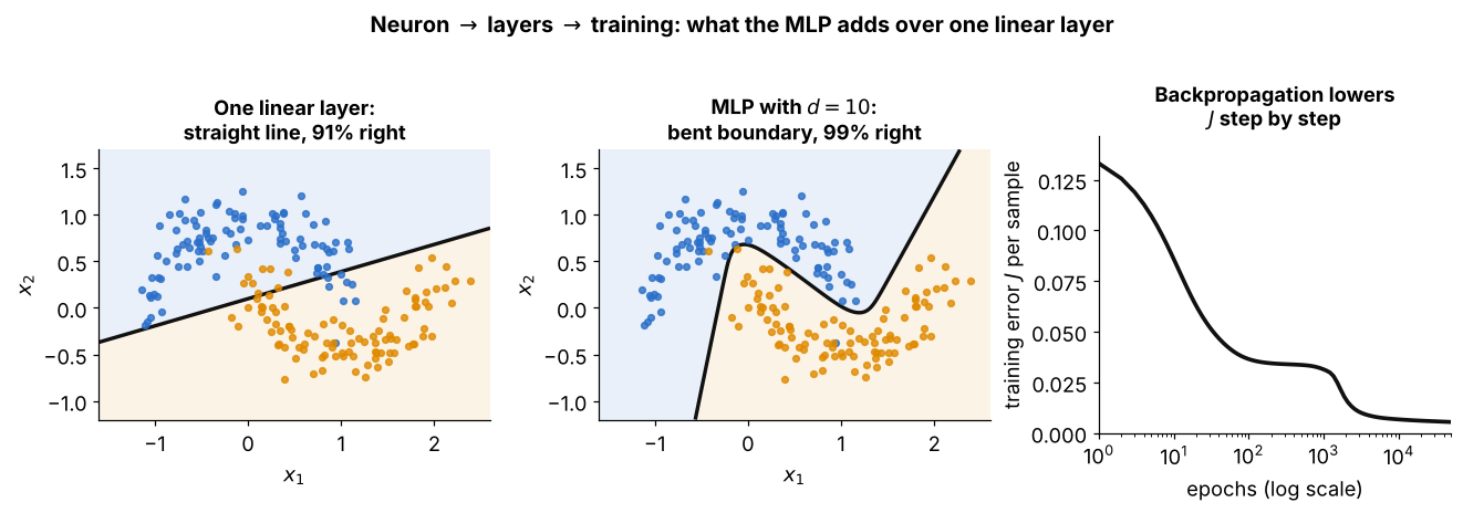
The three parts of this topic on one data set, how to read it:
- left: one linear layer trained by least squares, with targets , can only draw the straight line , and gets 91% of the two moons right
- middle: an MLP with sigmoid hidden neurons bends the boundary around the moons and gets 99% right
- right: the MLP weights have no closed form, so backpropagation lowers the training error step by step, with flat stretches where training almost stalls
- so the order is neuron and layers, then least squares for one layer, then backpropagation for hidden layers