Introduction
Instead of solving for the least squares weights in one go, the network can also obtain them by iteratively adjusting : start anywhere, and after each training sample nudge the weights a little in the direction that lowers the error. This is gradient descent, and for a single linear layer it gives the simple LMS (least mean square) rule.
Main idea
Move the weights downhill on the error bowl: $\mathbf{w}\Leftarrow\mathbf{w}-\eta\nabla J(\mathbf{w})$. For $J=E\{e^2\}$ the gradient is $-2E\{e\,\mathbf{x}\}$, estimated from one sample as $-2e_i\mathbf{x}_i$. This gives the LMS rule $\mathbf{w}\Leftarrow\mathbf{w}+\eta(t_i-y_i)\mathbf{x}_i$, which moves toward the least squares solution $(\mathbf{X}\mathbf{X}^T)^{-1}\mathbf{X}\mathbf{t}^T$. The decision boundary $\mathbf{w}^T\mathbf{x}=0$ of one layer is always a line, plane or hyperplane.
Overview
The symbol means "replace the old value by the new one", one update per sample.
Step 1: gradient descent
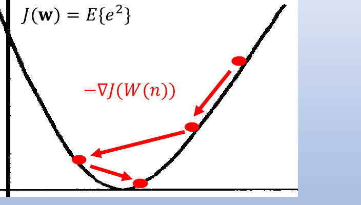
The gradient is the vector of partial derivatives, one per weight. It points uphill, in the direction where the error grows fastest. So step the other way:
Reading the figure:
- each red dot is the current , and each arrow is one step
- on a steep part of the bowl the gradient is large, so the step is long
- near the bottom the gradient is small, so the steps get shorter and the weights settle
- the label is the downhill direction at the weights after updates, so here counts steps, not inputs
The learning rate is a small positive number that sets the step size:
- too small, and learning is very slow
- too large, and the steps overshoot the bottom of the bowl, as the long arrow across the bowl shows, and can blow up
Step 2: gradient of the mean square error
Differentiate . By the chain rule, the derivative of is , times the derivative of the inside, :
Setting this to zero gives back from Least Squares Single Layer Network. Gradient descent never solves it directly, it only uses the gradient at the current .
Step 3: one sample at a time
The expected value is unknown. Estimate it from the current training sample alone:
Put this into , and absorb the 2 into :
How to read the rule:
- if the output is too small (), add a bit of to , which makes bigger next time, since
- if the output is too big (), subtract a bit of
- if the output is right, nothing changes
- the arrow means that over many samples, settles near the least squares solution
- each single-sample step is a noisy guess of the true downhill direction, but the guesses are right on average, so with a small (often reduced over time) the weights settle near the bottom
Step 4: learning curve and decision boundary
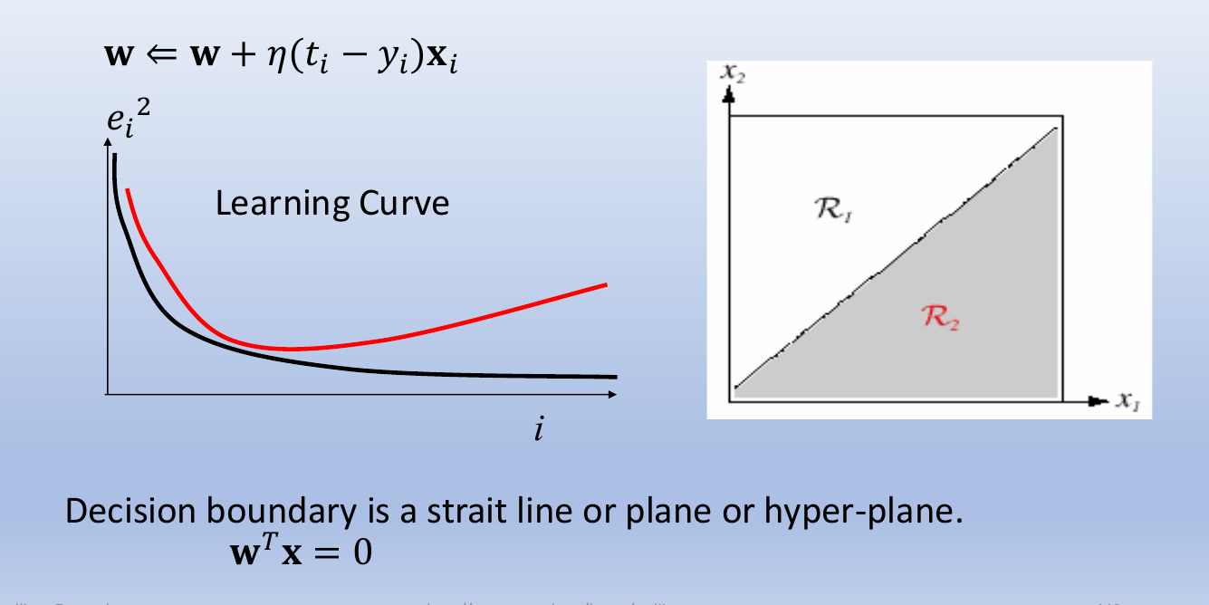
Reading the figure:
- left: the learning curve plots the squared error against the number of updates , and it falls quickly at first, then levels off as nears the bottom of the bowl
- the second curve falls and then rises again, the shape the error on new data can take, which is explained in Local Minima and Overfitting
- right: the input space is split into the decision regions and (where the network decides class 1 and class 2) by the boundary
Why the boundary is at 0: the class is read from the sign of the output, for example with target for one class and for the other. The boundary is where changes sign, so the decision boundary of a single layer network is always a straight line, plane or hyperplane:
Why do we need this
The LMS rule needs no matrix inverse and learns from a stream of samples. Most importantly, the same idea of "compute the error gradient, step downhill" still works when the network has nonlinear hidden layers, where no closed-form answer exists.
Next step
Backpropagation extends gradient descent to the hidden layers of an MLP.
Visual 1: LMS paths on the error bowl
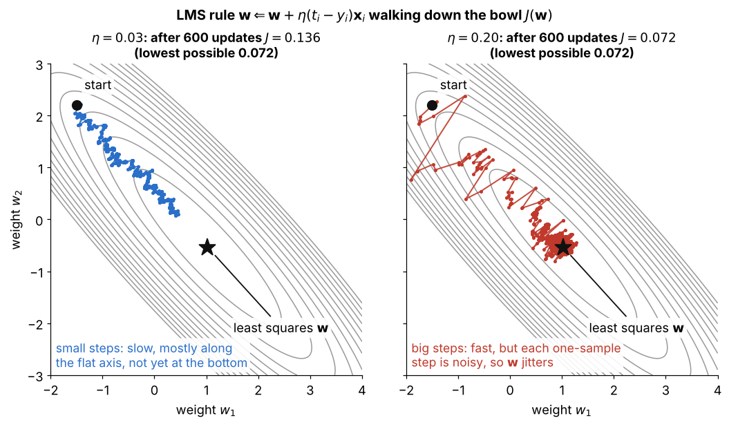
Same bowl as in Least Squares Single Layer Network, each dot is one update with one random sample:
- left, : steady but slow, after 600 updates , still far up the flat valley
- right, : reaches the bottom quickly, but each step follows one sample, so keeps jumping around the star instead of settling
- both paths cross the steep axis fast and move slowly along the flat one, as the eigenvalues of predict
- this is why is often reduced over time (Step 3): big steps first, small steps near the bottom
Visual 2: one LMS update
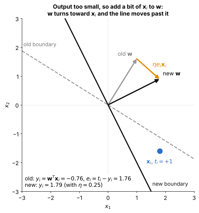
How to read it:
- the boundary is (no bias here), and has target but sits on the negative side with
- the error is , so the rule adds (orange) to
- the new leans toward , so grows to 1.79 and the boundary turns past
- this is the first case in Step 3, output too small so add a bit of , and the large makes it overshoot the target 1