Introduction
A two-layer MLP can represent almost any decision, but its best weights have no closed form, because the nonlinear sits between the layers. It is still trained by gradient descent, as long as the gradient of the error with respect to every weight can be computed. Backpropagation is the way to compute it: the output error is passed backward through the network, which gives each hidden neuron an effective error of its own.
Main idea
With $J=\frac12\sum_k(t_k-y_k)^2$, the chain rule gives the update rules $v_{kj}\Leftarrow v_{kj}+\eta(t_k-y_k)f'(q_k)z_j$ and $w_{ji}\Leftarrow w_{ji}+\eta\sum_k v_{kj}(t_k-y_k)f'(q_k)f'(q_j)x_i$. A hidden neuron has no target, so its error is the output errors sent back through the weights $v_{kj}$. Signals go forward to compute the outputs, and errors go backward to compute the updates.
Overview
Step 1: what two layers can represent
The two-layer MLP from Multilayer Perceptron Structure:
What it can do:
- any decision can be implemented by a two-layer network
- any function from input to output can be implemented in a two-layer network, given a sufficient number of hidden units, proper nonlinearities, and weights
Why a hidden layer adds so much: one neuron draws one straight boundary . A layer of hidden neurons draws several boundaries, and the nonlinear lets the output neuron combine them into regions of any shape.
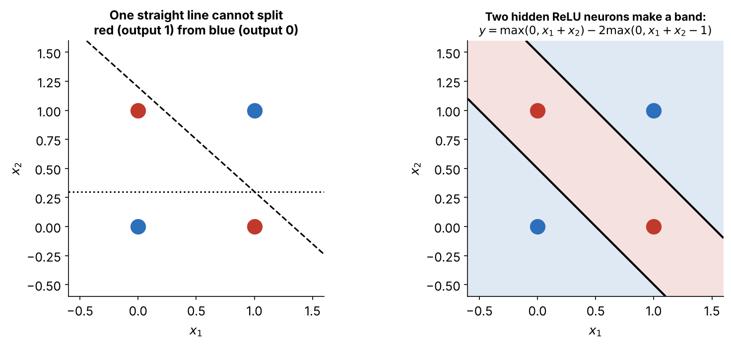
The classic case one layer cannot solve is XOR, output 1 when exactly one of two binary inputs is 1:
How it works:
- left: the two classes sit on opposite corners, so no single straight line separates them (the dashed and dotted lines are two failed tries)
- right: two hidden ReLU neurons and , where the is a bias, combined by a linear output
- rises with up to 1, then falls, so it is 0 at both blue corners and 1 at both red corners
- deciding red when keeps the band , between two parallel lines
- the bend in comes from the hidden ReLUs, and without it would be linear in and could not rise and then fall
- with more hidden neurons, can bend more times, so the boundary can take any shape
Step 2: central problem
Being able to represent a function is not the same as finding it:
- how to find the nonlinear function based on data is the central problem in network training
- the output neurons have targets , but the hidden neurons have none, so it is not obvious how to correct a hidden weight
- the power of backpropagation is that it computes an effective error for each hidden unit, and from it a learning rule for the hidden weights
- even if the network learns the training data perfectly, with zero training error, the machine learning problem may still not be solved (Local Minima and Overfitting)
Step 3: no analytical solution
The error to minimize, for the network output :
Here means , the squared length of the error vector, and and stand for all first-layer and all second-layer weights. To minimize , set . Unlike Least Squares Single Layer Network, this has no analytical solution, because the weights sit inside the nonlinear . But gradient descent only needs the gradient at the current weights for a given sample (here numbers the sample):
So the whole task is to compute and for every weight.
Step 4: scalar form
Use the scalar form of the weights to derive the learning formulas. Give a name to each weighted sum:
- hidden neuron : and
- output neuron : and
From here on, numbers the inputs again. The index letter tells the layer: is always a hidden neuron and is always an output neuron, so and are different sums, and and are slopes in different layers.
As in LMS Gradient Descent Learning, replace the average by the current sample alone. For that one sample, the error is the sum over the outputs, with a factor that cancels the 2 from differentiating a square and only rescales :
Writing out the hidden layer too:
Step 5: output layer gradient
The weight appears only inside , so it affects only output . The chain rule follows that one path, :
Each factor:
- : only the term contains , and its derivative is
- , because and only one term contains
Step 6: hidden layer gradient
The weight changes , which changes , which feeds every output through :
flowchart LR
    W["w_ji"] --> Q["q_j"] --> Z["z_j"]
    Z --> Q1["q_1 → y_1"]
    Z --> Q2["q_k → y_k"]
    Z --> Q3["q_c → y_c"]
    Q1 --> J["J"]
    Q2 --> J
    Q3 --> J
So the chain rule has three factors, and the first one sums over all outputs:
Each factor:
- , using Step 5 and
- , because
- , because
The first factor is the effective error of hidden neuron : the output errors , sent back through the same weights that carried forward.
Step 7: update rules
Step downhill, :
Put in Steps 5 and 6. The minus signs cancel:
How to read them:
- the output rule is the LMS rule again, with the hidden output as the input and an extra factor for the output activation
- both rules have the same shape: learning rate, times the error at the receiving neuron, times the slope there, times the signal coming in
- a short name for the error times the slope is the local gradient, and , so the rules become and
- bias weights follow the same rules: with and (Multilayer Perceptron Structure, Step 2), the bias updates are and
- the hidden rule uses the old , the ones that produced this output, so find every before changing any
Step 8: sigmoid slope
The rules need . For the sigmoid, whose output lies between 0 and 1:
Differentiate with the chain rule. The outer derivative is , and the inner one is :
Why the last form holds: split the fraction as . The first part is , and the second is , since .
What this gives:
- and , computed from outputs already found in the forward pass
- the slope is largest when and near 0 when is close to 0 or 1, so a saturated neuron hardly learns
For the other activations in Activation Functions:
- ReLU: for and for , so a neuron with a negative sum passes back no error for this sample
- linear output, : , so and the output rule is exactly the LMS rule
Step 9: two modes and two signals
The trained network, the multilayer perceptron, has two modes of operation:
- feedforward: present a pattern to the input units and pass (feed) the signals through the network, layer by layer, to get the outputs, with no cycles
- learning: present an input pattern and modify the weights to reduce the distance between the computed output and the desired output, which is supervised learning (learning from inputs paired with their desired outputs)
This learning algorithm is called backpropagation.
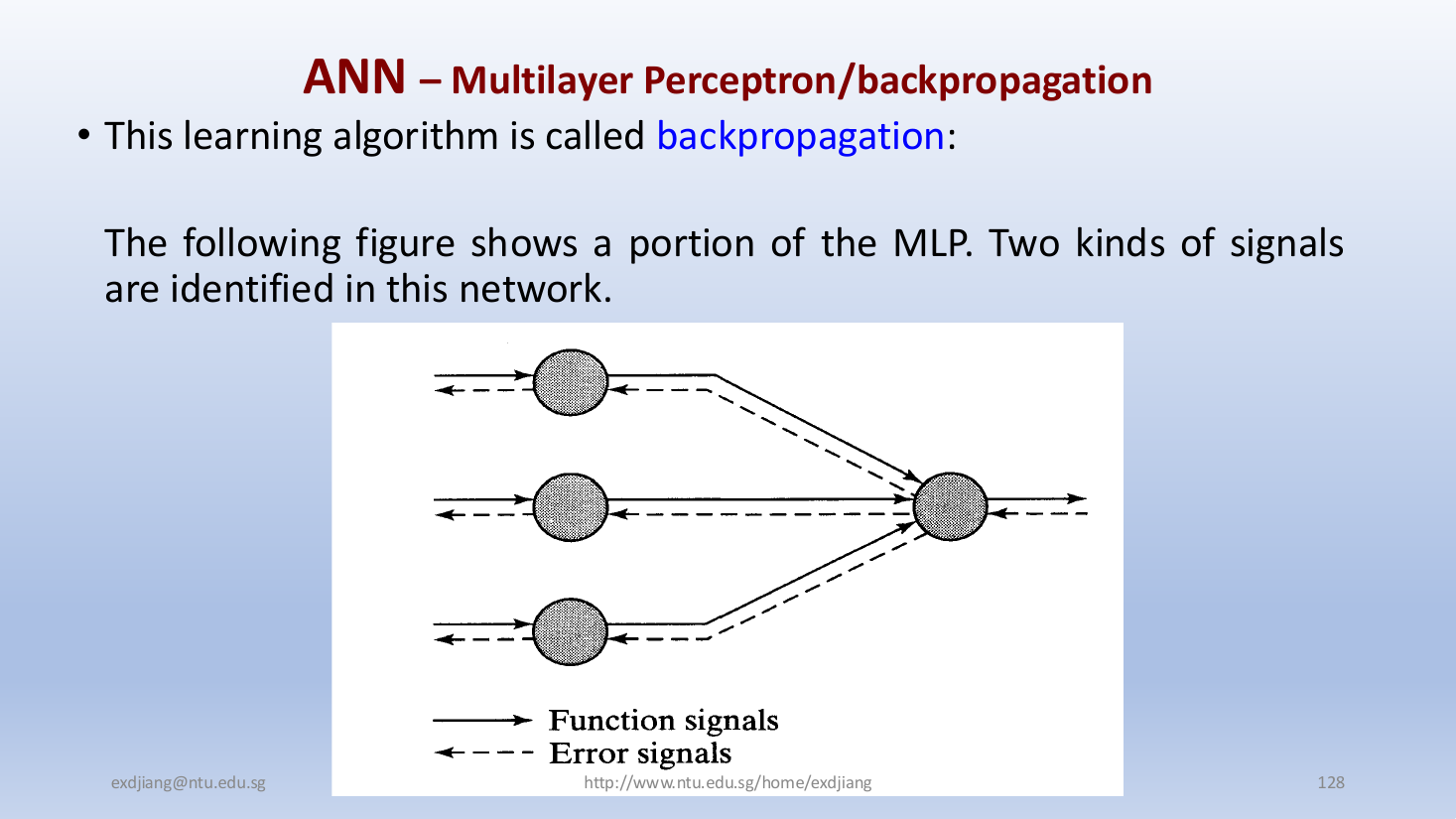
A portion of the MLP shows its two kinds of signals:
- function signals (solid arrows) flow forward, from the inputs through the weights to the outputs, which is Step 4
- error signals (dashed arrows) flow backward, from the output errors through the same weights to the hidden neurons, which is the sum in Step 6
Step 10: training procedure
Assume there are training samples . Here counts samples, not inputs. The procedure:
- Initialization: with no prior information, pick the weights from a uniform distribution with zero mean, and a variance chosen so that the standard deviation of the activation signals lies at the change between the linear part of the sigmoid (its nearly straight middle) and its saturated parts (the flat ends), where the slope is still large. Larger weights give larger sums , which is why the weight variance sets where lands. Random weights are needed because with all weights equal, every hidden neuron would compute the same output and get the same update, and they would never become different
- Presentation of training samples: present an epoch (one pass over all training samples), and for each sample do a forward and a backward computation
- Forward computation: apply to the input layer and present the target at the output layer for comparison, then compute the activation signals () and function signals (, ) layer by layer
- Backward computation: compute the local gradients and then , from the output back toward the input, and adjust the weights with Step 7. Find every before changing any , since must use the weights that produced this output
- Iteration: repeat steps 3 and 4 with new epochs until a stopping criterion is met
Why do we need this
Backpropagation is what makes multilayer networks trainable. It gives every hidden weight a gradient at a cost similar to one forward pass, because each weight is used once going forward and once going back, and it is still the training method for CNNs and Transformers.
Next step
Local Minima and Overfitting covers the stopping criterion and what can still go wrong after training.
Visual 1: errors sent back through the weights
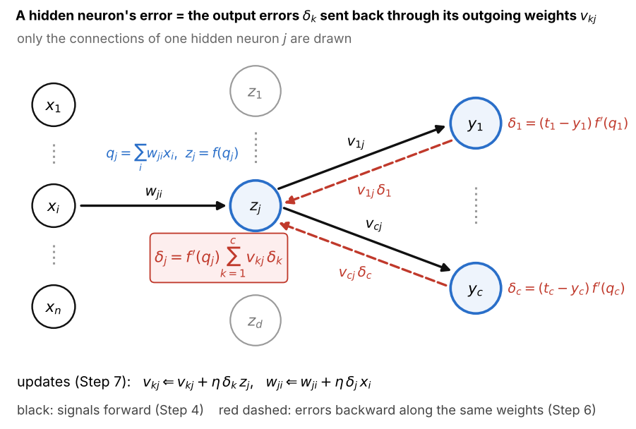
Steps 4 to 7 for one hidden neuron, how to read it:
- only the connections of hidden neuron are drawn: comes in through , and goes out to every output through
- forward (black): and , and each output then computes from all the
- each output has a target, so its local gradient is direct:
- backward (red dashed): each travels back along the same weight , so neuron collects and multiplies by its own slope, (Step 6)
- a large hands back much of the error of output and a negative flips its sign, and both updates of Step 7 then read times times the incoming signal
Visual 2: hidden lines make a region
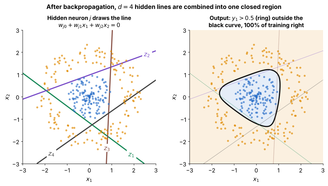
How to read it:
- a 2-4-1 sigmoid MLP trained by backpropagation on an inner disc (blue) and a ring (orange) around it
- left: each hidden neuron only splits the plane with one line
- right: the output neuron weights the four by and squashes the sum, so the black boundary follows pieces of the hidden lines (dotted) and closes around the disc
- no single line separates these classes, but several combined do, which is the idea of Step 1