Introduction
Before training many layers, look at the simplest case: one layer, one linear output, . "Training" means choosing so the output is close to the target . For this network the best weights have a closed-form answer, the least squares solution.
Main idea
Minimize the mean square error $J(\mathbf{w})=E\{(t-\mathbf{w}^T\mathbf{x})^2\}$. It is a quadratic bowl in $\mathbf{w}$ with only one minimum, found by setting the gradient to zero: $E\{\mathbf{x}\mathbf{x}^T\}\mathbf{w}=E\{\mathbf{x}t\}$. With the samples as the columns of $\mathbf{X}$ and the targets in the row $\mathbf{t}$, this gives $\mathbf{w}=(\mathbf{X}\mathbf{X}^T)^{-1}\mathbf{X}\mathbf{t}^T$.
Overview
The whole note is one chain:
The sizes: and are , with the constant input 1 counted as one of the entries, is (one sample per column), and is (one target per sample). In this note there is one output, so each sample has a single target , and bold is the row of all of them. The index numbers the samples.
Step 1: error of one layer
A single layer network with a single output and a linear activation:
where includes the constant input 1, so includes the bias (Neuron Model). With a target output , the error of the output is:
For classification, the target is a class code, for example for one class and for the other, and the class is read from the sign of .
Step 2: mean square error
Square the error, so positive and negative misses both count, and average over the data. means the expected value, the average over all input and target pairs:
How the expansion works:
- , as for
- , since is a number
- , because is a number and equals its own transpose
- is fixed, so it moves outside
Step 3: only one minimum
is a quadratic (second order) function of : a constant, a term linear in , and a term with twice. So it has only one minimum point.
The picture in one dimension, with one sample:
- is a parabola in
- its minimum is at , where the error is zero
- the bowl opens upward because can never be negative
- in more dimensions the parabola becomes a bowl, with one bottom as long as is invertible, the same condition that lets Step 5 compute
- if is not invertible, for example with fewer samples than inputs (), the bowl has a flat valley and many give the same smallest error
- the bowl's axes are the eigenvectors of and its steepness along each axis is the eigenvalue, so along a direction with a tiny eigenvalue the bowl is almost flat, the weight there is poorly fixed by the data, and gradient descent moves slowly along it
- with suitable targets for two classes, the least squares weight vector points the same way as the LDA direction
Step 4: least squares solution
The optimal weights minimize the mean square error, so set the gradient to zero. Two gradient rules, the vector forms of and :
- for a symmetric , and is symmetric (why: , and its derivative by is , which is when )
does not depend on , so its gradient is zero. Then:
This gives the least mean square solution of .
Step 5: from training samples
The expected values are unknown. With training samples and their targets , replace each expected value by an average:
Collect the samples as columns and the targets as a row:
Why the sums become matrix products:
- is () times (), and multiplying column by row it equals , so
- is () times (), which is each column times its target , added up, so
Put these into Step 4. The is on both sides and cancels:
The output for a new input is then:
using and the fact that is symmetric. This form gives the output straight from the training samples and targets. The matrix is called the pseudo-inverse of .
Names: "least squares", "least mean square solution" and "least square method" all mean this one closed-form answer. The LMS rule in the next note is an iterative way to reach the same answer.
Why do we need this
It shows that training is just minimizing an error, and that for one linear layer the minimum is unique and can be written down. The inverse is costly for large inputs and has no counterpart for nonlinear layers, which is why an iterative method is needed next.
Next step
LMS Gradient Descent Learning reaches the same weights by small corrections, one sample at a time.
Visual 1: least squares boundary and the LDA direction
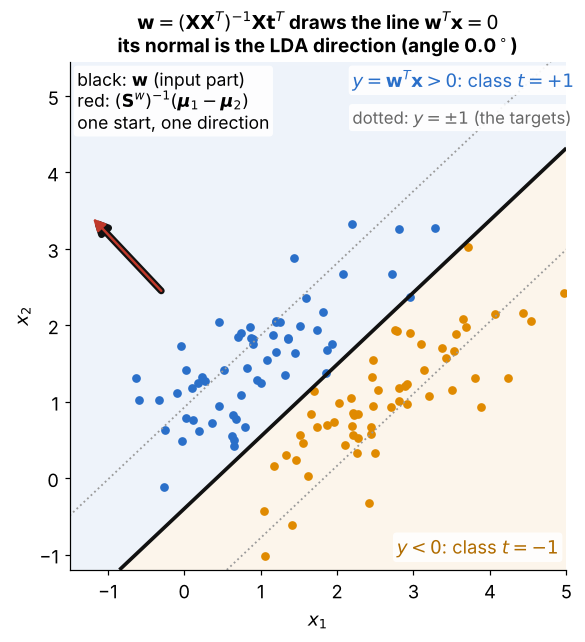
How to read it:
- 60 samples per class with targets and , and includes the constant input 1
- the black line is where , and the dotted lines are , the values the outputs are pulled toward
- the input part of (thick black arrow) and (thin red arrow) start at the same point and lie on top of each other, the LDA claim at the end of Step 3
- 1 of the 120 training samples falls on the wrong side
Visual 2: error bowl and its axes
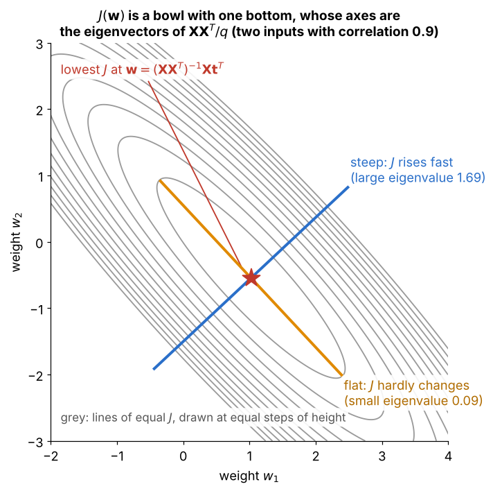
How to read it:
- two inputs with correlation 0.9, 80 samples and no bias, so can be drawn over the plane of
- the grey ellipses are lines of equal , one step of height apart, around one bottom at (red star)
- the two coloured lines, drawn the same length, are the eigenvectors of : along the blue one (large eigenvalue) the ellipses are packed close, so climbs fast
- along the orange one (small eigenvalue) the ellipses are far apart, so barely changes and the data fixes poorly, the nearly flat valley of Step 3