Introduction
Backpropagation reduces the training error step by step, but two things can still go wrong. Training can get stuck before it finds a good solution, and a network that fits the training data perfectly can still do badly on new data. These are the central problems of machine learning, and the reason later networks were designed the way they are.
Main idea
A two-layer network can approximate any continuous function, but this does not mean training finds that function. Gradient descent can stop in a **local minimum**, under-fitting the training data. Even a perfect fit to the training data can fail on new data, which is **over-fitting** or poor generalization. A validation set shows when to stop training.
Overview
Training can fail in two opposite ways:
| Problem | Training error | Error on new data | Cause |
|---|---|---|---|
| local minimum (under-fitting) | stays high | high | gradient descent stops in the wrong dip |
| over-fitting (poor generalization) | low | high | the network learns details of the training samples that do not hold for new ones |
Two more causes to keep in mind:
- a network with too few hidden neurons can also under-fit, because it cannot represent the function at all
- over-fitting is more likely when the network has many parameters (Multilayer Perceptron Structure, Step 3) compared with the number of training samples
Step 1: stopping criterion
Training is repeated epoch after epoch, so it needs a rule for when to stop. The stopping criterion can be:
- a fixed number of iterations
- the point where the rate of change of the average error is small enough
- a third criterion, the minimum of the validation error, comes in Step 3
Step 2: problem of local minima
For a single linear layer, the error is a bowl with one minimum (Least Squares Single Layer Network). With nonlinear hidden layers, the error surface has many dips.
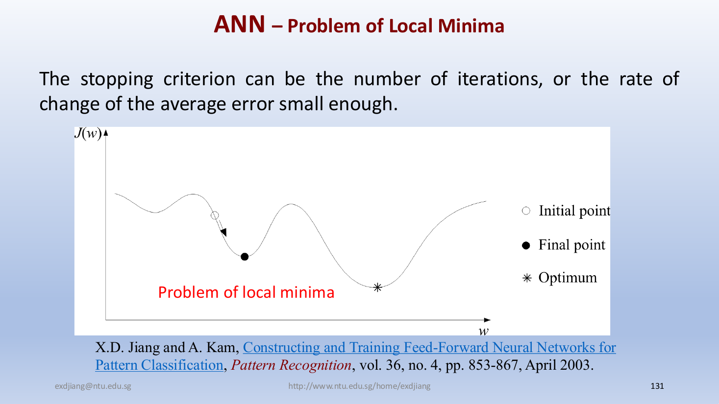
What the figure shows:
- gradient descent from the initial point (circle) goes downhill and stops at the bottom of the nearest dip, the final point (dot)
- that local minimum has a higher error than the true optimum (star) further along
- the gradient there is zero, so the update is zero and plain gradient descent cannot climb out
- where training ends depends on where it starts, which is why the initialization matters
- the result is under-fitting: the network does not even fit its training data well
Step 3: learning curves
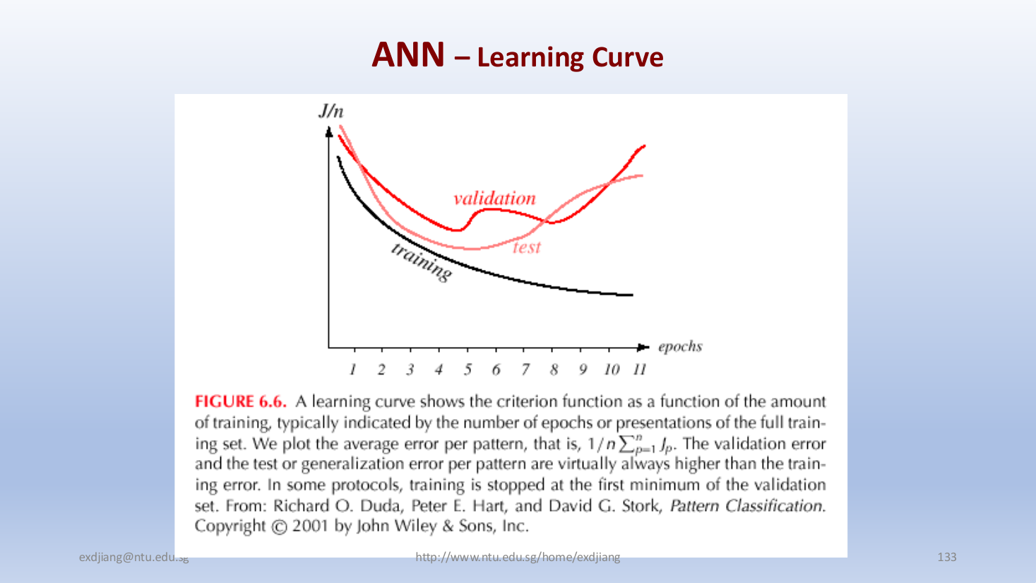
The three curves, plotted against the number of epochs, where is the average error per training pattern ( counts patterns here):
- training error: high before training starts, and it keeps getting smaller through the learning process
- test error, on an independent test set: always higher than the training error, and it can decrease as well as increase
- validation error: measured on a separate validation set, and used to decide when to stop
Why the test error rises again:
- early on, the network learns the patterns shared by all samples of a class, so both errors fall
- later, it starts to learn the details and noise of its particular training samples, which do not hold for new samples
- this is the misleading information of Objectives of Dimensionality Reduction: patterns that look discriminative in the training samples but are not in the population
- the training error keeps falling, but the error on new data rises: this is over-fitting, the generalization problem
The remedy: stop training at a minimum of the error on the validation set, normally the first clear minimum, since later dips come after the network has started to over-fit. Stopping there keeps the network from over-fitting, so it keeps its power to generalize to new data.
A separate validation set is needed because once a set is used to choose when to stop, its error is no longer a fair guess of the error on new data. So the test set is kept untouched for the final check, and the validation set is a third part held back from the training samples.
Step 4: conclusions on neural networks
The three facts to remember:
- universal approximators: any nonlinear continuous function can be approximated arbitrarily closely by a two-layer perceptron, provided a large enough number of nodes is used
- local minima: this does not mean the network will be trained to that solution, so it can under-fit the training data
- poor generalization: even if learning is powerful enough to find the solution, it is a solution on the training data, and over-fitting the training data is the central issue of machine learning
This answers the question from Backpropagation: zero training error does not solve the machine learning problem, because what matters is the error on new data.
Why do we need this
These problems explain the history of neural networks. Large MLPs over-fit badly and were hard to train, which is what CNNs were designed to fix by restricting how the weights are used.
Next step
Convolutional Neural Network CNN starts from exactly these problems.
Visual 1: over-fitting seen in the input space
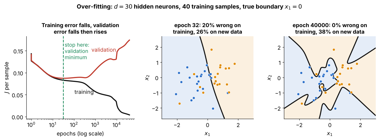
How to read it:
- 40 noisy training samples of two classes (blue, orange) that truly differ only in , and an MLP with hidden neurons, far more weights than samples
- left: the training error keeps falling over 40,000 epochs, but the error on 2,000 validation samples is lowest at epoch 32 and then rises
- middle: stopped at the validation minimum, the boundary is close to the true line , and 26% of new samples are wrong, near the 25% that the best boundary gets on this data
- right: trained to the end, the boundary twists around single training points, 0% wrong on training but 38% wrong on new data
- this is over-fitting, and the remedy of Step 3 is to stop at the validation minimum
Visual 2: plateau or local minimum
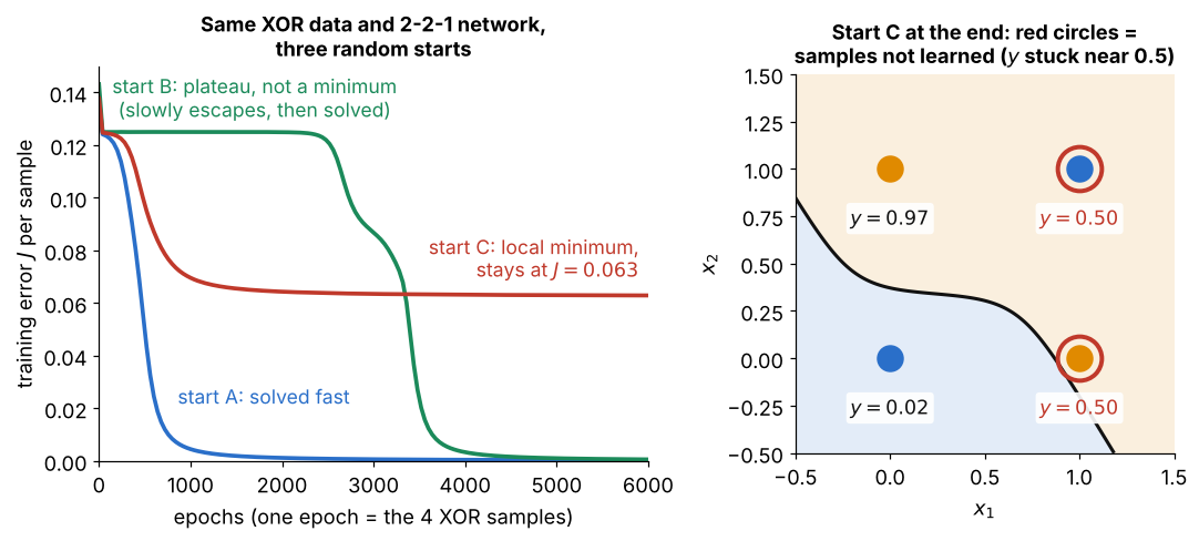
Three starts on the four XOR samples, same 2-2-1 sigmoid network and :
- these three of 40 random starts were picked on purpose to show the three outcomes (of all 40, 32 reached and 8 stayed high)
- start A (blue) is solved within about 800 epochs
- start B (green) sits for about 2,500 epochs at , where every output is about : a plateau, where the gradient is tiny but not zero, so it escapes in the end
- start C (red) settles at and stays there, a local minimum: on the right, two XOR samples still give (circled), so the network never learns them
- so where training ends depends on where it starts, the problem of Step 2