Introduction
A multilayer perceptron (MLP) is a stack of neuron layers, where every neuron in one layer feeds every neuron in the next. This note sets up the notation for a two-layer MLP, writes its output in scalar, vector and matrix form, counts its parameters, and shows why the activation function must be nonlinear.
Main idea
$z_j=f(\mathbf{w}_j^T\mathbf{x})$ and $y_k=f(\mathbf{v}_k^T\mathbf{z})$, or for whole layers $\mathbf{y}=f\left(\mathbf{V}^Tf(\mathbf{W}^T\mathbf{x})\right)$. If $f$ were linear, the two layers would collapse into one: $\mathbf{y}=(\mathbf{W}\mathbf{V})^T\mathbf{x}=\mathbf{U}^T\mathbf{x}$. So the activation must be nonlinear, at least for the hidden neurons.
Overview
The sizes of a two-layer MLP with inputs, hidden neurons and outputs:
Each arrow is "multiply by a weight matrix, then apply to every entry".
Step 1: architecture and notation
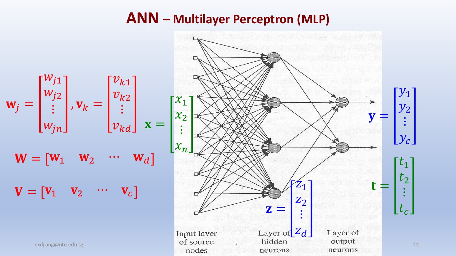
The layers:
- the input layer holds the source values , and does no computing
- the hidden layer has neurons with outputs , called hidden because they are neither input nor output
- the output layer has neurons with outputs , compared with the targets
The weights of each neuron are stored as one column, and the columns of a layer side by side make its weight matrix:
How to read the indices:
- joins input to hidden neuron , and column of holds all the weights coming into hidden neuron
- joins hidden neuron to output , and column of holds all the weights coming into output
- the first index is always the receiving neuron, the second the sending one
- so is and is
- this puts in row , column of , the reverse of the subscript order
- the input layer does no computing, so this network has two layers of computing neurons and is called a two-layer network
Step 2: outputs from inputs
The same computation in three forms.
Scalar form, one weight at a time:
Vector form, one neuron at a time. The sum is the dot product of column with :
Matrix form, a whole layer at once. Row of is , so entry of is . Apply to each entry:
These sums start at and , so as written they have no bias. To include it, use the trick from Neuron Model: add a constant to and to , each with its own weight and . Then grows to and to , which is where the in Step 3 comes from.
Step 3: counting parameters
The trainable parameters are the weights and biases. Count neuron by neuron, then layer by layer:
- a neuron has one weight for each connection coming into it, plus one bias
- a hidden neuron receives all inputs, so it has parameters, and the hidden layer has
- an output neuron receives all hidden outputs, so it has parameters, and the output layer has
- the input nodes only pass values on, so they have no parameters
Without biases the count is . The two differ by , one bias per computing neuron, so always say whether the biases are included.
Step 4: why the activation must be nonlinear
Suppose the activation is linear, . Then does nothing, and:
Explaining each equals sign:
- the first removes , since
- the second uses backwards, so
- the last names the product , an matrix
What this means:
- a multilayer network with linear activations is just the same as a single layer network with weights
- any number of linear layers collapses the same way, because a product of matrices is one matrix
- a single linear layer can only draw straight boundaries ()
- so to design a multilayer network, the activation function must be nonlinear, at least for the hidden neurons
The output neurons may still be linear, for example when the network has to produce any real number.
Why do we need this
The matrix form shows that a layer is just "multiply by a weight matrix, then apply ", which is also the core of CNNs and Transformers. The collapse argument shows that the nonlinearity is the whole reason to have more than one layer.
Next step
Before training two layers, Least Squares Single Layer Network finds the best weights for one linear layer.
Visual 1: each layer as one matrix product
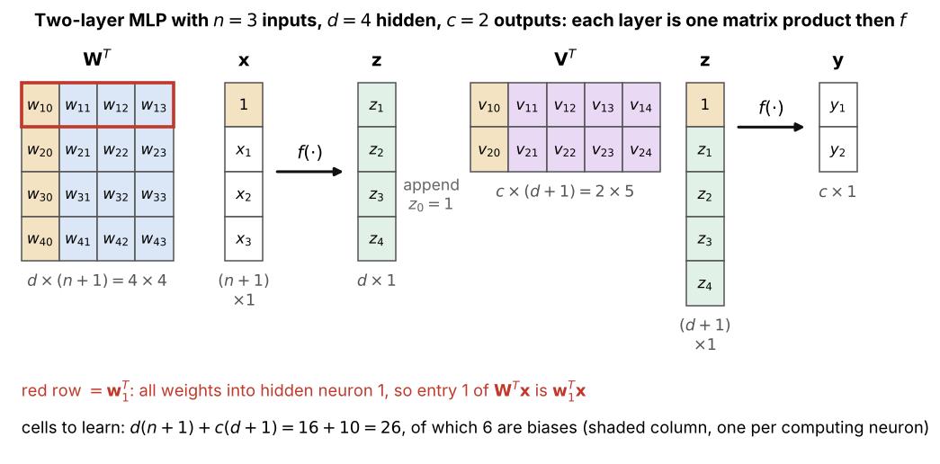
Steps 2 and 3 for , , , how to read it:
- row of holds every weight into hidden neuron , so each entry of is one dot product
- the shaded first columns hold the biases and , which multiply the constants and
- gives only , and the constant is appended before the second layer
- the inner sizes must match: has columns for , and has columns for with its 1
- counting the cells gives , the formula of Step 3, of which are biases
Visual 2: linear layers collapse, ReLU bends
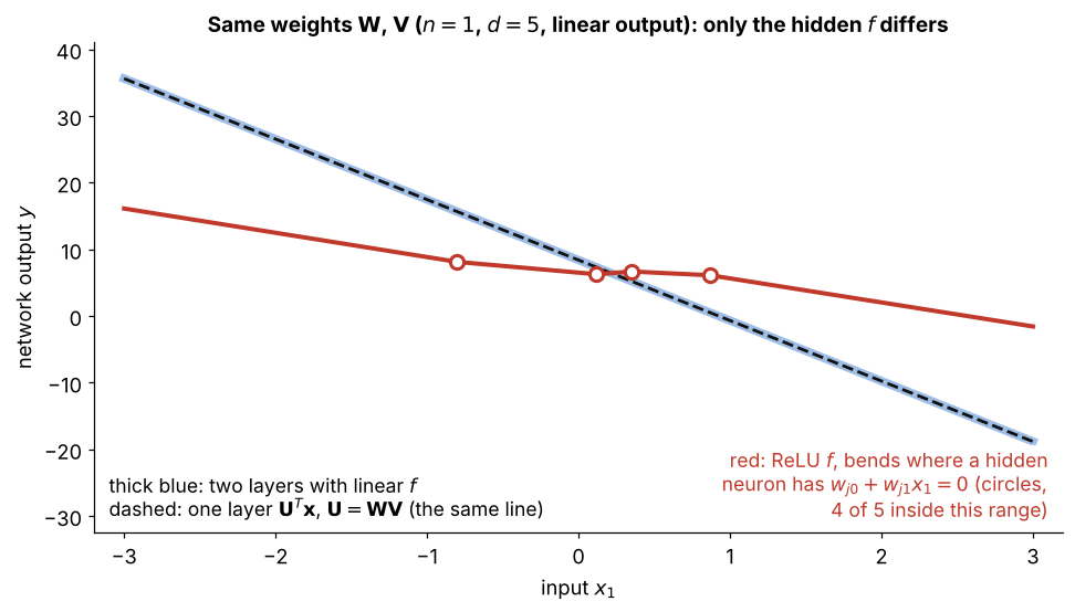
How to read it:
- both curves use the same random weights, one input, hidden neurons with biases and a linear output neuron
- with a linear (thick blue) the output is a straight line, exactly the one layer with (dashed), as Step 4 proves
- with ReLU (red) each hidden neuron switches on or off where , and the output bends there (4 of the 5 switch points fall inside the plotted range)
- these bends are what let more hidden neurons build more complex shapes, which no stack of linear layers can do