Computed Torque Control

Introduction

Computed torque control is Control Law Partitioning applied to a robot. Robot dynamics are highly non-linear, and the joints are coupled. The model based portion cancels these non-linear terms, so the closed loop system is linear and decoupled.

The control law uses the Robot Dynamic Model:

$$M(\theta )\ddot{\theta }+C(\theta ,\dot{\theta })\dot{\theta }+g(\theta )=\tau$$

Single link robot

For the single link robot $m{l}^2\ddot{\theta }+mgl\cos \theta =\tau$, use $\tau =\alpha v+\beta$ with:

$$\alpha =m{l}^2\beta =mgl\cos \theta$$

This gives $\ddot{\theta }=v$. The servo portion is $v={\ddot{\theta }}_d+k_v\dot{e}+k_{p}e$, with $e={\theta }_d-\theta$. So:

$$\ddot{e}+k_v\dot{e}+k_{p}e=0$$ $$\boxed{\tau =m{l}^2({\ddot{\theta }}_d+k_v\dot{e}+k_{p}e)+mgl\cos \theta }$$

The torque is computed in this form and applied to the motor.

Multi input, multi output robot

A robot with $n$ joints is a MIMO system. Now $v$ and $\beta$ are $n\times 1$ vectors, and $\alpha$ is an $n\times n$ matrix. Choose:

$$\alpha =M(\theta )\beta =C(\theta ,\dot{\theta })\dot{\theta }+g(\theta )$$

Then the closed loop is $\ddot{\theta }=v$. This is a set of $n$ separate unit masses:

$${\ddot{\theta }}_1=v_1,{\ddot{\theta }}_2=v_2,\dots ,{\ddot{\theta }}_n=v_n$$

So you can design each $v_i$ separately.

PD computed torque

The servo law for each joint:

$$v_i={\ddot{\theta }}_{id}+k_{vi}{\dot{e}}_i+k_{pi}{e}_i{e}_i={\theta }_{id}-{\theta }_i$$

In vector form, with diagonal gain matrices $K_v$ and $K_p$:

$$v={\ddot{\theta }}_d+K_v\dot{E}+K_{p}E$$

The error equation is:

$$\ddot{E}+K_v\dot{E}+K_{p}E=0$$

The full control law is:

$$\boxed{\tau =M(\theta )({\ddot{\theta }}_d+K_v\dot{E}+K_{p}E)+C(\theta ,\dot{\theta })\dot{\theta }+g(\theta )}$$

flowchart LR
    TD["θ_d, θ_d-dot, θ_d-ddot"] --> SV["Servo<br/>v = θ_d-ddot + K_v E-dot + K_p E"]
    SV -->|"v"| MB["Model based<br/>τ = M v + C θ-dot + g"]
    MB -->|"τ"| R["Robot"]
    R -->|"θ, θ-dot"| SV
    R -->|"θ, θ-dot"| MB

PID computed torque

Add an integral term to remove the steady state error, with $K_I$ also diagonal:

$$\tau =M(\theta )({\ddot{\theta }}_d+K_v\dot{E}+K_{p}E+K_I\int Edt)+C(\theta ,\dot{\theta })\dot{\theta }+g(\theta )$$ $$\ddot{E}+K_v\dot{E}+K_{p}E+K_I\int Edt=0$$

Example

Design a PD computed torque controller for the two link polar robot with $m=2$ kg. The resonant frequency is 20 rad/s.

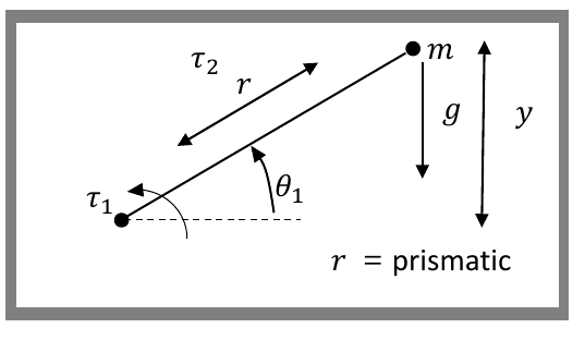
Note

The first example slide calls this robot the "2-link polar robot". The next slides call it a "2-link planar robot", but the model (with prismatic joint $r$) is the same two link polar robot.

Step 1: dynamic model (with $g=9.8$ m/s², so $mg=19.6$)

$$M(\theta )=\left[\begin{array}{cc}2r^2& 0\\ 0& 2\end{array}\right]C(\theta ,\dot{\theta })\dot{\theta }=\left[\begin{array}{c}4r\dot{r}{\dot{\theta }}_1\\ -2r{\dot{\theta }}_1^2\end{array}\right]g(\theta )=\left[\begin{array}{c}19.6r\cos {\theta }_1\\ 19.6\sin {\theta }_1\end{array}\right]$$

Step 2: model based portion

$$\alpha =\left[\begin{array}{cc}2r^2& 0\\ 0& 2\end{array}\right]\beta =\left[\begin{array}{c}4r\dot{r}{\dot{\theta }}_1+19.6r\cos {\theta }_1\\ -2r{\dot{\theta }}_1^2+19.6\sin {\theta }_1\end{array}\right]$$

Step 3: servo portion

$$v_1={\ddot{\theta }}_{1d}+k_{v1}{\dot{e}}_1+k_{p1}{e}_1{v}_2={\ddot{r}}_d+k_{v2}{\dot{e}}_2+k_{p2}{e}_2$$

with $e_1={\theta }_{1d}-{\theta }_1$ and $e_2=r_d-r$.

Step 4: gains

The characteristic equations are $s^2+k_{vi}s+k_{pi}=0$. Compare with $s^2+2\zeta {\omega }_{n}s+{\omega }_n^2=0$:

• ${\omega }_n\le 0.5\times 20=10$ rad/s, so choose ${\omega }_n=10$ rad/s
• $k_{p1}=k_{p2}={\omega }_n^2=100$
• $k_{v1}=k_{v2}=2\zeta {\omega }_n\ge 20$, so that $\zeta \ge 1$ (choose 20 for critical damping)

Step 5: control law

$$\left[\begin{array}{c}{\tau }_1\\ {\tau }_2\end{array}\right]=\left[\begin{array}{cc}2r^2& 0\\ 0& 2\end{array}\right]\left[\begin{array}{c}{\ddot{\theta }}_{1d}+k_{v1}{\dot{e}}_1+k_{p1}{e}_1\\ {\ddot{r}}_d+k_{v2}{\dot{e}}_2+k_{p2}{e}_2\end{array}\right]+\left[\begin{array}{c}4r\dot{r}{\dot{\theta }}_1+19.6r\cos {\theta }_1\\ -2r{\dot{\theta }}_1^2+19.6\sin {\theta }_1\end{array}\right]$$

With $k_p=100$, the damping ratio is $\zeta =k_v/20$. The lecture shows animations of this robot for $\zeta =0.1$ (underdamped), $\zeta =10$ (overdamped) and $\zeta =1$ (critically damped).