Robot Dynamic Model

Introduction

To use model based (non-linear) control, you need a dynamic model of the robot. You can derive robot dynamics from the Lagrange equation of motion, which uses the energies of the mechanical system. The model is the base of Computed Torque Control.

Lagrange equation

The Lagrangian $L$ is kinetic energy minus potential energy:

$$L=K-P$$ $$\boxed{\frac{d}{dt}\frac{\partial L}{\partial \dot{\theta }}=\tau +\frac{\partial L}{\partial \theta }}$$

This is Newton's law, $\frac{d}{dt}(\text{momentum})=\text{force}$, written with energies.

Single link robot

The mass $m$ is at the end of a link of length $l$.

$$K=\frac{1}{2}m{v}^2=\frac{1}{2}m{l}^2{\dot{\theta }}^{2}P=mgy=mgl\sin \theta$$ $$L=\frac{1}{2}m{l}^2{\dot{\theta }}^2-mgl\sin \theta$$ $$\frac{\partial L}{\partial \dot{\theta }}=m{l}^2\dot{\theta }\frac{\partial L}{\partial \theta }=-mgl\cos \theta$$ $$\frac{d}{dt}(m{l}^2\dot{\theta })=\tau -mgl\cos \theta$$ $$\boxed{m{l}^2\ddot{\theta }+mgl\cos \theta =\tau }$$

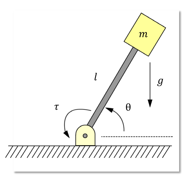
This is non-linear. The moment of inertia is $m{l}^2$, and there is a gravity torque $mgl\cos \theta$ from the load.

Two link polar robot

Joint 1 is revolute (${\theta }_1$) and joint 2 is prismatic ($r$). The mass $m$ is at the end of the link.

$$K=\frac{1}{2}m{r}^2{\dot{\theta }}_1^2+\frac{1}{2}m{\dot{r}}^{2}P=mgr\sin {\theta }_1$$

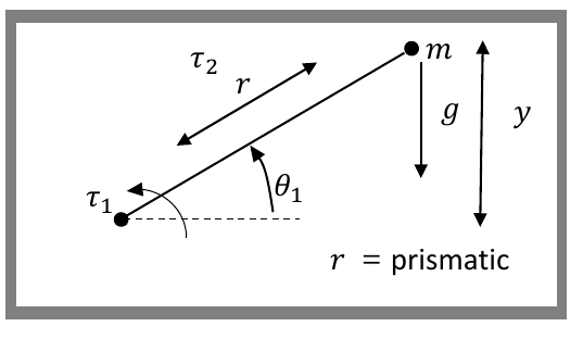
With $\theta =[{\theta }_1,r{]}^T$ and $\tau =[{\tau }_1,{\tau }_2{]}^T$, the Lagrange equation gives:

$$m{r}^2{\ddot{\theta }}_1+2mr\dot{r}{\dot{\theta }}_1+mgr\cos {\theta }_1={\tau }_1$$ $$m\ddot{r}-mr{\dot{\theta }}_1^2+mg\sin {\theta }_1={\tau }_2$$

In vector form:

$$\left[\begin{array}{cc}m{r}^2& 0\\ 0& m\end{array}\right]\left[\begin{array}{c}{\ddot{\theta }}_1\\ \ddot{r}\end{array}\right]+\left[\begin{array}{c}2mr\dot{r}{\dot{\theta }}_1\\ -mr{\dot{\theta }}_1^2\end{array}\right]+\left[\begin{array}{c}mgr\cos {\theta }_1\\ mg\sin {\theta }_1\end{array}\right]=\left[\begin{array}{c}{\tau }_1\\ {\tau }_2\end{array}\right]$$

General form

For a robot with $n$ degrees of freedom:

$$\boxed{M(\theta )\ddot{\theta }+C(\theta ,\dot{\theta })\dot{\theta }+g(\theta )=\tau }$$

• $\theta$ is the $n\times 1$ vector of joint positions, and $\tau$ is the $n\times 1$ vector of joint inputs
• $M(\theta )$ is the $n\times n$ manipulator mass matrix. It is always symmetric and positive definite, so it is always invertible
• $C(\theta ,\dot{\theta })\dot{\theta }$ has all the terms that depend on joint velocity. A term like $mr{\dot{\theta }}_1^2$ comes from centrifugal force (square of one joint velocity). A term like $2mr\dot{r}{\dot{\theta }}_1$ comes from Coriolis force (product of two different joint velocities)
• $g(\theta )$ has all the terms with the gravity constant $g$

Two link planar robot

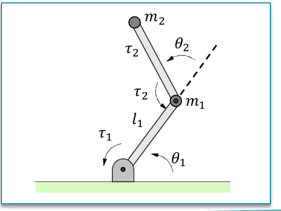
Each robot has a different model. For a two link planar robot (both joints revolute), with $c_2=\cos {\theta }_2$, $s_2=\sin {\theta }_2$, $c_{12}=\cos ({\theta }_1+{\theta }_2)$:

$$M(\theta )=\left[\begin{array}{cc}(m_1+m_2)l_1^2+m_2{l}_2^2+2m_2{l}_1{l}_2{c}_2& m_2{l}_2^2+m_2{l}_1{l}_2{c}_2\\ m_2{l}_2^2+m_2{l}_1{l}_2{c}_2& m_2{l}_2^2\end{array}\right]$$ $$C(\theta ,\dot{\theta })\dot{\theta }=\left[\begin{array}{c}-m_2{l}_1{l}_2({\dot{\theta }}_2^2+2{\dot{\theta }}_1{\dot{\theta }}_2)s_2\\ m_2{l}_1{l}_2{\dot{\theta }}_1^2{s}_2\end{array}\right]$$ $$g(\theta )=\left[\begin{array}{c}(m_1+m_2)g{l}_1{c}_1+m_{2}g{l}_2{c}_{12}\\ m_{2}g{l}_2{c}_{12}\end{array}\right]$$

Note

This slide writes the first entry as $m_2{l}_1{l}_2({\dot{\theta }}_1^2+2{\dot{\theta }}_1{\dot{\theta }}_2)s_2$. A later slide (dual rate computed torque) writes it as $-m_2{l}_1{l}_2{s}_2{\dot{\theta }}_2^2-2m_2{l}_1{l}_2{s}_2{\dot{\theta }}_1{\dot{\theta }}_2$. The later form is the correct one, and this note uses it.