Degradation and Restoration Process

Overview of Process

flowchart LR

F["F(u,v)<br/>Spectrum of the original image"] --> M["Multiply"]
H["H(u,v)<br/>Blur or degradation function"] --> M

M --> HF["H(u,v)F(u,v)"]
HF --> ADD["Add"]
N["N(u,v)<br/>Noise spectrum"] --> ADD

ADD --> G["G(u,v) = HF + N<br/>Observed degraded image"]

G --> BQ{"Is blur (H) present?"}

BQ -- "NO, H = 1" --> NQ{"Is noise (N) present?"}
NQ -- "NO, IDEAL CASE" --> CLEAN["No restoration needed"]
NQ -- "YES" --> NT{"Which noise type?"}

NT --> NR["Random noise"]
NR --> NF["Spatial smoothing filters<br/>Mean or geometric mean"]

NT --> NI["Impulse noise"]
NI --> MED["Median for salt-and-pepper<br/>Max for pepper<br/>Min for salt"]

NT --> NP["Periodic noise"]
NP --> PEAK["Find isolated peaks<br/>in the Fourier spectrum"]
PEAK --> REJ["Notch-reject or band-reject<br/>removes those frequencies"]

BQ -- "YES" --> EST["Estimate the degradation function H"]

EST --> OBS["{Observation}<br/>Compare a strong observed subimage Gs<br/>with an estimated clean subimage F̂s"]
EST --> EXP["{Experimentation}<br/>Image a known impulse Aδ<br/>H = G / A"]
EST --> MODEL["{Mathematical modelling}<br/>Derive H from motion, optics,<br/>or atmospheric physics"]

OBS --> HEST["Estimated degradation function H"]
EXP --> HEST
MODEL --> HEST

HEST --> NS{"Is noise (N) significant?"}
NS -- "YES" --> WIEN["Wiener filter<br/>Use H and noise statistics"]
NS -- "NO" --> HS{"Is H zero or very small<br/>at some frequencies?"}
HS -- "NO" --> INV["Inverse filter<br/>F̂ = G / H"]
HS -- "YES" --> PINV["Pseudo-inverse<br/>Avoid division when H is small"]

CLEAN --> FHAT["F̂(u,v)<br/>Estimated original spectrum"]
NF --> FHAT
MED --> FHAT
REJ --> FHAT
INV --> FHAT
PINV --> FHAT
WIEN --> FHAT

FHAT --> IFT["Inverse Fourier transform"]
IFT --> OUT["f̂(x,y)<br/>Estimated original image"]

LEG["Lowercase letters: spatial domain<br/>Uppercase letters: Fourier domain<br/>Hat: an estimate of the original"]
LEG -.-> G

Links: Noise-only Restoration · Periodic Noise · Estimating Degradation Function · Inverse Filtering · Wiener Filtering

Model of Imaging Chain

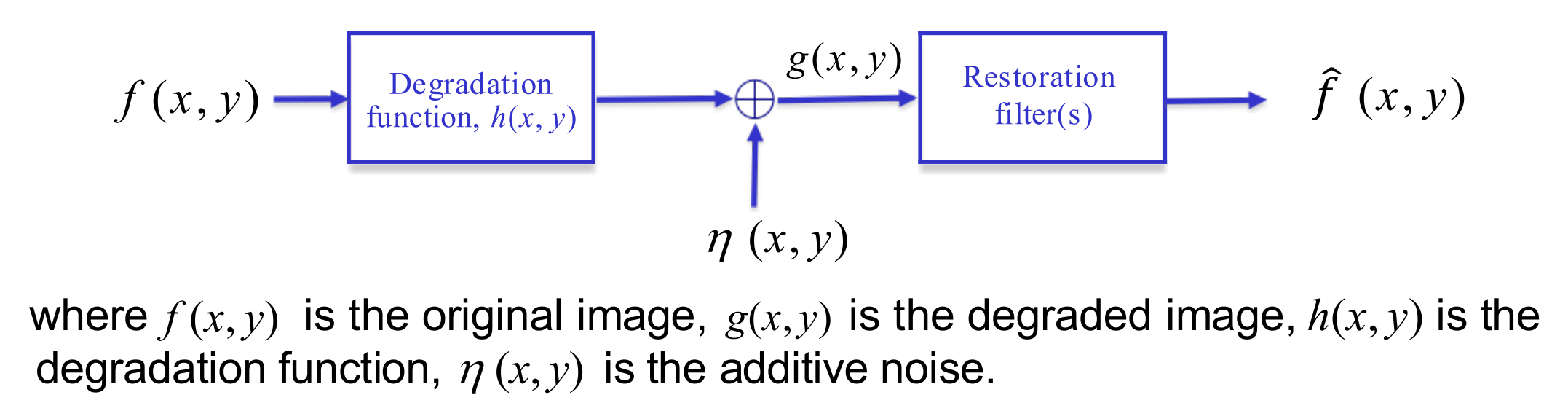
• This whole process in the image above is to model the whole imaging chain, from the lens (optics), motion (camera or scene moving), the medium (atmospheric turbulence, transmission interference, etc)

Objective

The objective of restoration is to obtain an estimate $\hat{f}(x,y)$ which is as close as possible to the original image $f(x,y)$.

Components

• degredation function is also called a point spread function or PSF
• it is the result of light hitting multiple pixels in a camera, instead of just one
• which causes the image to have destroyed information
• the noise function is a random value that's added to every pixel independent of the scene which comes from electronics, sensors or thermal effects
• The restoration filter is called $r(x,y)$ or $R(u,v)$ in frequency domain
• this is the main thing we need to derive
• the more information we have about the degredation function $h(x,y)$ and our additive noise $\eta (x,y)$, the better our restoration is to our true image

If our degradation function, $h(x,y)$ is a linear, space-invariant process, the degraded image can be modeled as:

$$g(x,y)=h(x,y)\ast f(x,y)+\eta (x,y)$$

When looking at the frequency domain, we get:

$$G(u,v)=H(u,v)F(u,v)+N(u,v)$$

Sequence of Solving

1. Model the degradation, giving $H(u,v)$
2. Model the noise statistically, giving $S_{\eta }(u,v)$ or the variance
3. Choose a criterion, which such as minimum mean square error
4. Solve for the $R(u,v)$ that optimises that criterion, given 1 and 2

3 Assumptions about the noise function above

1. Spatial Stationarity

• the noise statistics do not depend on the pixel position

1. Signal Uncorrelatedness

• the noise is uncorrelated with the underlying image, $E\{\eta (x,y)f(x,+i,y+j)\}=0$

1. Amplitude Statistics

• the gray level value of the noise component can be modeled as a random variable, characterized by a probability density function (PDF)

Autocorelation of Noise Field

$$E\{\eta (x,y)\eta (x+i,y+j)\}=\delta (i,j)$$

• we can model noise that is uncorrelated across pixels as white noise
• where power spectral density (PSD) of $\eta (x,y)$ is a constant
• PSD just tells us how much power a signal has at each frequency

Noise Models

• spatial correlation and amplitude distribution describe 2 different properties of noise
• the white noise assumption specifies how noise samples are related across pixels, whereas a PDF specifies the probability of each noise amplitude at a single pixel
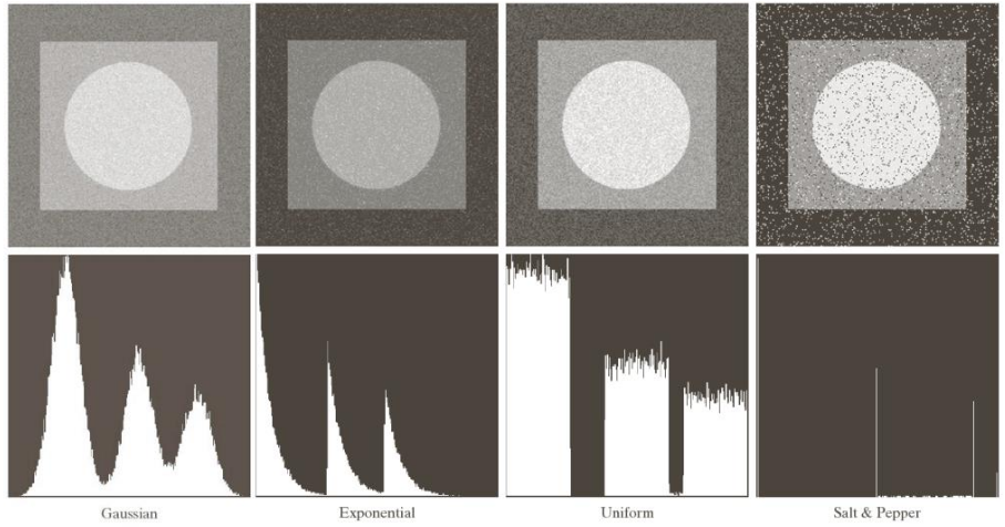
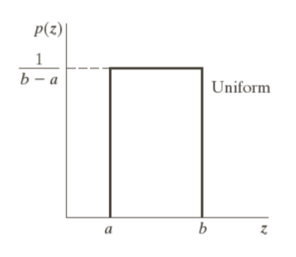
• under the additive, signal-independent model, we next compare four commonly used amplitude distributions: Gaussian, Exponential, Uniform and Impulse.

Gaussian Noise

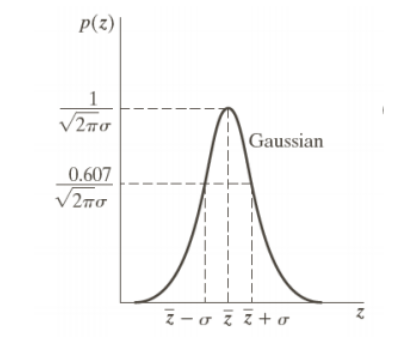
Gaussian noise is also called normal noise. It is represented as:

$$p(z)=\frac{1}{\sqrt{2\pi }\sigma }{e}^{-\frac{(z-\mu {)}^2}{2{\sigma }^2}}$$

• where $z$ represents gray level, $\mu$ is the mean, and $\sigma$ is the standard deviation, and ${\sigma }^2$ is the variance of $z$

Exponential Noise

$$p(z)=\{\begin{array}{ll}a{e}^{-az}& z\ge 0\\ 0& z<0\end{array}$$

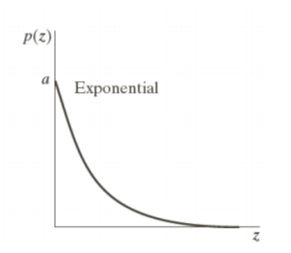
• where $a>0$
• The mean and variance of $z$ are:

$$\mu =\frac{1}{a}{\sigma }^2=\frac{1}{a^2}$$

Uniform Noise

$$p(z)=\{\begin{array}{ll}\frac{1}{b-a},& a\le z\le b\\ 0,& \text{otherwise}\end{array}$$ $$\mu =\frac{a+b}{2}{\sigma }^2=\frac{(b-a{)}^2}{12}$$

Impulse Noise

$$p(z)=\{\begin{array}{ll}{P}_a,& z=a\\ P_b,& z=b\\ 0,& \text{otherwise}\end{array}$$ $$\mu =a{P}_a+b{P}_b{\sigma }^2=a^2{P}_a+b^2{P}_b-{\mu }^2$$

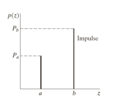
How different types of noise looks