Introduction
The Gaussian discriminant function needs the inverse of an covariance matrix, which hides what each estimated number does. Writing it with the Eigen-Decomposition of the covariance matrix turns it into a simple sum over dimensions. This form shows clearly why small eigenvalues learned from training data make the classifier unreliable.
Main idea
$g_i(\mathbf{x})=-\frac{1}{2}\sum_{k=1}^{n}\frac{(z_k-\bar{z}_k)^2}{\lambda_k}+b_i$, where $z_k-\bar{z}_k=\boldsymbol{\phi}_k^T(\mathbf{x}-\boldsymbol{\mu}_i)$. Each dimension is weighted by $1/\lambda_k$. The smallest training eigenvalues are far smaller than the true variances, so these dimensions get huge, wrong weights and dominate the decision.
Overview
The same function in two forms, with the class covariance :
Steps 1 and 2 say why we need the second form, Steps 3 and 4 derive it, and Steps 5 and 6 use it to find the problem.
Step 1: Gaussian discriminant function
If the data of every class is Gaussian, the optimal (Bayes) decision evaluates, for each class :
and picks the class with the largest .
Reminders of the ideas this uses (each is explained in its own note):
- is the covariance matrix of class : its diagonal entries are the variances of the features, its off-diagonal entries are their covariances, and it is symmetric (Principal Component Analysis, Step 4)
- is the class density, here a multivariate Gaussian, and is the prior probability of the class (Bayes Decision and Classifiers)
- picking the class with the largest gives the lowest error, and taking keeps the same order (MAP Decision Rule)
Where the formula comes from and what each part means:
- it is for a Gaussian , with the terms that are the same for every class dropped
- the first part is the squared Mahalanobis distance between and the class mean , scaled by (Mahalanobis and Euclidean Distance)
- collects the terms that do not depend on , such as and , and the user can also add a constant to it, which moves the threshold to lower the error rate of one class at the price of the other classes
- depends on the same eigenvalues as the first part, so when they are corrected later, this term changes with them
- the two parts pull in opposite ways: a tiny makes larger, which raises the score of class , while the distance term divides the offset along axis by ; for a new sample with a normal offset, grows much faster than , so the distance term wins and the sample is pushed away from its own class
- some forms leave out the , which only multiplies every by 2, so with scaled to match the decision is the same
Step 2: estimates replace the truth
The problem:
- human knowledge cannot give the class mean and covariance matrix of the population
- they can only be estimated (learned) by the machine from the available training samples
- these estimates may differ from the truth, so for a robust and accurate classifier we must study how the estimation errors affect the accuracy
Why the usual form makes this hard:
- depends on all estimated entries of at once, so it is hard to see which estimate causes which problem
- the covariance matrix is symmetric, so its eigenvectors give an orthogonal basis of the -dimensional space
- eigen-decomposition uses this basis to split the problem into independent one-dimensional pieces
Step 3: eigen-decomposition
Recall, for a symmetric with orthonormal eigenvectors as the columns of :
Apply it to the covariance of class : , with and . For simpler symbols, the class index is left off and , but they belong to class .
Step 4: derivation
First name the projections onto the eigenvectors, because the last line uses them:
Substitute into the quadratic term:
Explaining each line:
- line 2 uses the inverse of a product, , which reverses the order
- line 3 uses , so also
- line 4 groups the outer factors, using
- line 5: the vector has entries , and , so
So the discriminant function becomes:
Step 5: scalar form in the eigenspace
What the formula says:
- in the eigenspace spanned by the , the inverse of an matrix becomes a simple sum of scalar terms
- term is the squared distance from the class mean along , divided by , which is the variance of class along (an eigenvalue of a covariance matrix is the variance along its eigenvector, Principal Component Analysis, Step 6)
- so each dimension is measured in units of its own spread, with weight
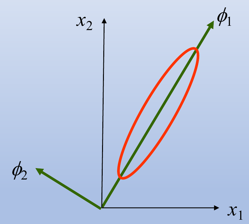
- the ellipse in the figure is a contour of the class (a line of equal density), and lies along its long axis, where is large and a step counts little, and lies along the short axis, where is small and a step counts a lot
Step 6: problem of small eigenvalues
The problem is now evident if some eigenvalues are unreliable, especially if some eigenvalues are small and close to zero: a tiny gives a huge weight .
Reading the figure:
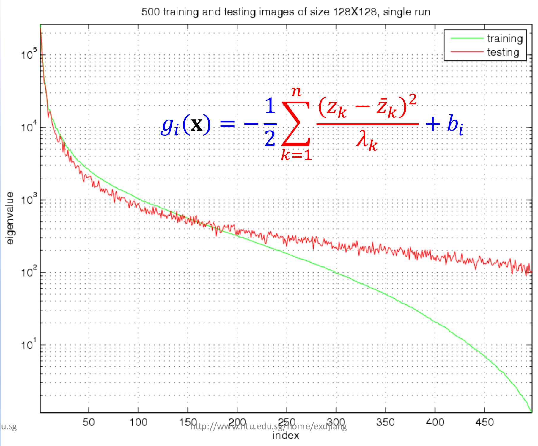
- there are 500 training images of size , so , but only about 500 eigenvalues can be nonzero, which is why the index stops near 500
- the green curve is the eigenvalues learned from the training images
- the red curve is the variance of new (testing) images along the same eigenvectors
- for the largest eigenvalues (small ) the curves are close, with the training values even a little above the testing ones, so these dimensions are reliable
- for small eigenvalues (large ) the training eigenvalues fall far below the testing variances
- so is far too large in these dimensions, and they dominate with misleading weights
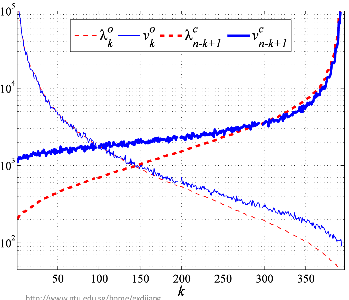
The same problem appears for two classes, (o for the object class) and (c for its counterpart class):
- (thin dashed red) are the eigenvalues of class , and (thin solid blue) are the variances of new samples of along the same eigenvectors
- the curves of class (thick lines) are drawn in the reverse order of , only so that both classes fit on one plot with their small eigenvalues at opposite ends
- in both classes, the variances of new samples are much larger than the small eigenvalues learned from the training data
Why the small training eigenvalues are too small:
- the eigenvectors of the smallest eigenvalues are, by construction, the directions in which these particular training samples happen to spread the least
- new samples were not used to choose these directions, so they have no reason to be as tight there, and they spread more
- with training samples, has at most nonzero eigenvalues (the rank argument in PCA Reconstruction, Step 4), so when many eigenvalues are exactly zero although the population still varies in those directions, and does not even exist
What goes wrong in a decision:
- a new sample of class moves a normal amount along an unreliable
- that small move is divided by a tiny , so the sample gets a huge distance from its own class mean
- becomes very negative, and the sample can be assigned to another class
So the dimensions of the small eigenvalues are unreliable, and they must be corrected (regularized) or removed.
LDA Variants describes NDA, which treats zero within-class spread as the most useful direction. Step 3 there explains why the two views differ.
Why do we need this
It turns the vague "remove unreliable dimensions" into a precise target: the eigenvectors with small eigenvalues of the class covariance matrices. Every solution that follows changes the weights of exactly these dimensions.
Next step
Eigenvalue Regularization keeps all dimensions and makes the small eigenvalues larger.
Visual 1: one tiny eigenvalue dominates the sum
How to read it:
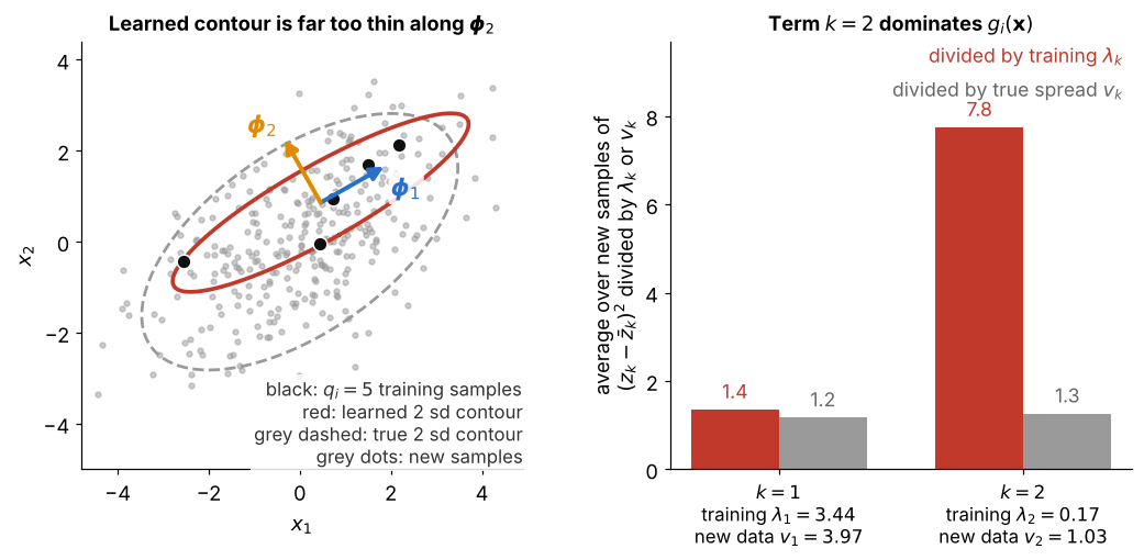
- a class with true variances 4 and 1 is learned from only samples (black dots), and the red ellipse is the contour of the learned
- is the spread of new samples along : along the training is close to , but along the training is 6 times smaller than
- this training set was picked on purpose: over 2,000 random sets of 5 samples, has median 3.6 and is above 7 in a quarter of them
- right: for new samples of this class, term of averages 7.8 (red), against about 1 when divided by (grey)
- so the weight makes new samples look far from their own class mean, the failure described in Step 6