Motion Control Schemes

Introduction

There are several control techniques for a manipulator:

• Linear control (classical control theory) is the simplest method
• Non-linear control, such as computed torque control, uses a model of the robot

This note covers the linear method. For the non-linear method, see Non-linear Control Methods.

Classical joint control

In classical joint control, each joint of the robot is treated as a simple joint servomechanism. A controller $G_c(s)$ drives a DC servo motor, which turns the link through a gear train.

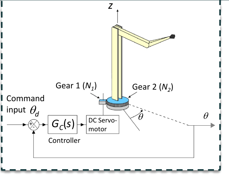
In the early days of robotics, independent joint control was popular. Each joint is a separate single input, single output (SISO) system, so the closed loop analysis is decoupled and you can use classical techniques.

How it works

1. Model one joint (DC motor, gear train and link) as a transfer function $G_p(s)$
2. Add a controller $G_c(s)$ in a unity feedback loop
3. Choose the controller type (P, PD or PID) and its gains
4. Check the stability and performance of the closed loop

flowchart LR
    TD["θ_L^d(s)"] --> SUM(("Σ"))
    SUM -->|"E(s)"| GC["G_c(s)<br/>controller"]
    GC -->|"V_a(s)"| GP["G_p(s)<br/>motor and link"]
    GP --> TL["θ_L(s)"]
    TL -->|"−"| SUM

Closed loop transfer function

From the block diagram:

$$E(s)={\theta }_L^d(s)-{\theta }_L(s)$$ $${\theta }_L(s)=G_p(s)G_c(s)({\theta }_L^d(s)-{\theta }_L(s))$$

The open loop transfer function is $G(s)=G_c(s)G_p(s)$. The closed loop transfer function is:

$$\boxed{\frac{{\theta }_L(s)}{{\theta }_L^d(s)}=\frac{G_c(s)G_p(s)}{1+G_c(s)G_p(s)}=\frac{G(s)}{1+G(s)}}$$

Limitation

Robot dynamics are highly non-linear, and the joints are coupled. The linear approach makes approximations so that each joint is a linear system. These approximations limit the performance of the system.