Introduction
Attention appears in two places in a Transformer, and each place has several attention heads. Before any attention can relate tokens to each other, each token is turned into three vectors with three different jobs: a query (what this token is looking for), a key (what this token offers to be matched against), and a value (what this token contributes if it is chosen). They come from three learnable linear projections of the same input, shared by all tokens.
Main idea
$\mathbf{Q}=\mathbf{X}\mathbf{W}_q$, $\mathbf{K}=\mathbf{X}\mathbf{W}_k$, $\mathbf{V}=\mathbf{X}\mathbf{W}_v$, or for each token row $\mathbf{q}_i=\mathbf{x}_i\mathbf{W}_q$, $\mathbf{k}_i=\mathbf{x}_i\mathbf{W}_k$, $\mathbf{v}_i=\mathbf{x}_i\mathbf{W}_v$. All tokens share the same three weight matrices, so every learnable parameter goes through all tokens and is learned from all of them, which is a $1\times1$ convolution of a CNN.
Projection has the same meaning as in Visual Data Dimensionality Reduction: each column of is a direction, and each entry of is the coordinate of the token along it. The difference is that these directions are learned by backpropagation, are not orthonormal, and need not reduce the dimension.
Overview
The sizes, with tokens of features:
Steps 1 and 2 show where attention is used. Steps 3 to 6 build , and .
Step 1: two kinds of attention
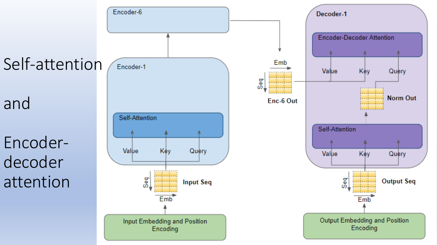
Reading the figure:
- self-attention (in every encoder and every decoder): the query, key and value all come from the same sequence, so the sequence pays attention to itself
- encoder-decoder attention (in every decoder): the key and value come from the output of the final encoder (Enc-6 Out), and the query comes from the decoder's own self-attention below it
- so each output word can look up the relevant input words
Step 2: multiple heads
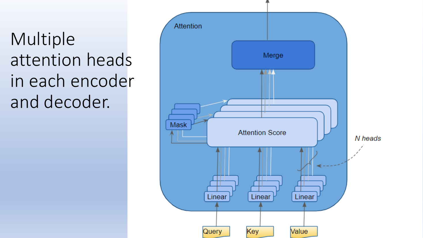
Each encoder and decoder has several attention heads. The figure labels the number of heads , and these notes call it , since is the number of tokens. Reading the figure:
- each head takes the query, key and value through its own linear layers, so each head has its own , ,
- each head computes its own attention scores, with an optional mask (used in the decoder)
- the outputs of the heads are concatenated side by side, and a learned linear layer (Merge) maps them back to width
- different heads can attend to different kinds of relation between tokens
The attention score is defined in the next note, Attention as Weighted Sum of Values, and the mask in its Step 3. The steps below build the query, key and value that it uses.
Step 3: three copies of each token
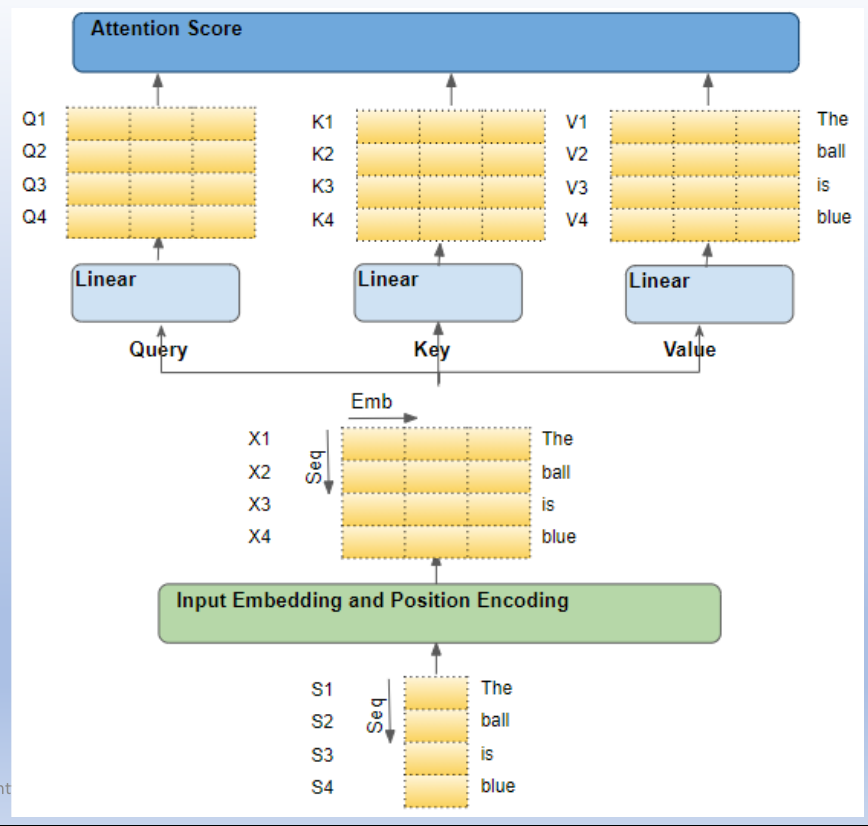
Take an English-to-Spanish translation, where the source sequence is "The ball is blue" and the target is "La bola es azul".
Reading the figure from the bottom:
- the four source words go through input embedding and position encoding, giving the rows of
- goes through three linear layers side by side
- this gives three copies of each token for self-attention: its query, its key and its value
Step 4: learnable linear projections
The input sequence (a matrix, one token per row) passes through three trainable linear layers. They produce three separate matrices, the Query, the Key and the Value:
Each row of these matrices is one token, here . Row of a product is row of times , so:
Step 5: shapes
With tokens of features:
- is
- each of , , is (it can also map to a different width)
- , and are , one row per token
- the weight matrices have no dimension of size , so the number of learnable parameters does not depend on the number of tokens, and the same layer works for a sequence of any length
Step 6: shared weights
All tokens use the same , and . To see the sharing, look at one entry of in the row form used here:
How to read it:
- is feature of token , and it uses only token 's own features
- the weight has no token index , so the same weight is used for every token
- so any single learnable parameter goes through all tokens, and is learned from all tokens
- this is exactly a convolution in a CNN, which applies the same small weight matrix at every position to mix the features (channels) of that position only: here each token is a position and its features are the channels
Step 7: tokens as columns
The same operations can be written with each token as a column, the convention of the earlier MLP notes. The tools needed:
- a row token is , and the same token as a column is , which is
- stacking the column tokens side by side gives , which is
- the transpose of a product reverses the order:
Practice
- which operations hold machine-learnt weights, and which do not?
- transpose both sides of each learnt row formula, and check the size of every matrix in the result
- rewrite the entry using the column-form matrices
- transpose the row formula for in Pointwise Feed-Forward Network from the inside out, and compare it with in the MLP notes
Why do we need this
The three projections let one token play different roles: asking, being matched, and contributing. They and the merge layer after the heads are the only learnable parts of an attention layer, so everything attention learns is stored in these linear layers, and weight sharing gives them the generalization of a CNN.
Next step
Attention as Weighted Sum of Values combines the queries, keys and values.
Visual 1: one weight matrix for every token
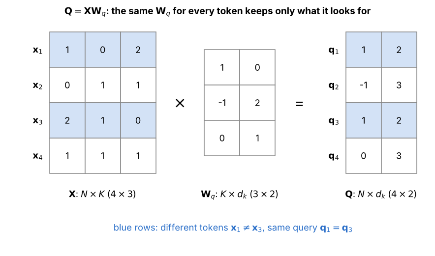
A small example with tokens of features, projected to width :
- every row of is multiplied by the same , so its 6 weights are used by all 4 tokens
- the blue rows and are different tokens, but both give
- so keeps only the part of a token along its own columns, what the query looks for, and drops the rest
- and are built the same way with their own matrices (Step 4 and Step 6)
Visual 2: coordinates along learned directions
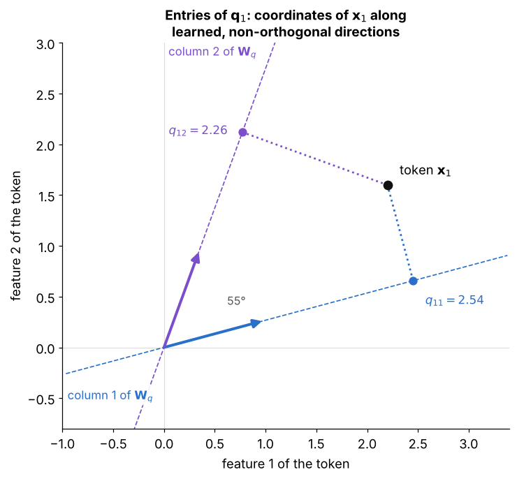
A token with features, and a whose two columns have length 1 but are apart:
- each dashed line is the direction of one column of
- dropping straight onto each line gives its coordinate there, so
- this is the same projection as in PCA, but the directions are learned by backpropagation and are not orthogonal
- and give each token two more sets of coordinates, along their own directions