Introduction
A Transformer works on vectors, so each input word (token) must first become a vector. Embedding turns each token into a feature vector, and position encoding adds where the token sits in the sequence. The vectors are stacked as the rows of one matrix . Each layer of an encoder then changes with a residual skip-connection around it.
Main idea
Each token's ID selects a learned feature vector, its embedding. A position vector is added, because attention by itself does not know the order of the tokens. Stacking the $N$ token vectors as rows gives $\mathbf{X}\in\mathbb{R}^{N\times K}$. Each attention and feed-forward layer is wrapped as "add the layer's input to its output, then normalize".
Overview
From words to the matrix that enters the first encoder:
Step 1: word IDs
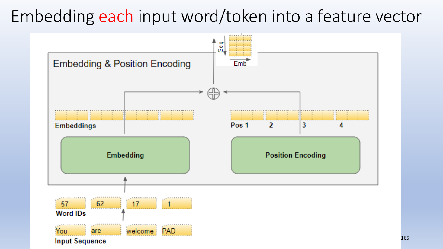
Reading the figure from the bottom, for the input sequence "You are welcome PAD":
- each word is looked up in a vocabulary to get a word ID, here 57, 62, 17 and 1
- "PAD" is a padding token that fills unused places, so that sentences of different lengths can be processed together in one batch as matrices of the same size (the layers themselves work for any number of tokens )
Step 2: embedding
Each word ID selects one row of a learned table. That row is the word's embedding, a feature vector of length .
What this gives:
- every word becomes a vector of the same length, whatever the word
- the table is learned in training, so words used in similar ways end up with similar vectors
- for an image, the tokens are small patches of the image instead of words
Step 3: position encoding
Attention by itself ignores order. Its output for token is a sum over all tokens, (see Attention as Weighted Sum of Values), and reordering the terms of a sum does not change it. So if the input tokens are shuffled, each token gets the same output as before, only in a shuffled row. "dog bites man" and "man bites dog" would give each word the same vector.
So a position encoding vector, one for each position , is added ( in the figure) to each embedding:
What the position vector is:
- a vector of length for each position, the same size as an embedding
- it is either a fixed pattern of sine and cosine waves of different frequencies, or a learned table with one row per position
- adding it works because the network learns to use both parts: the embedding part says which word, and the position part says where
The same word now has a slightly different vector at different positions, so later layers can use word order. This sum is the "embedding with time signal" in Encoder and Decoder Stacks.
Step 4: tokens as rows
The token vectors are stacked as the rows of a matrix:
What this means:
- row is token with its features, and column is feature across all tokens
- in the figures, the yellow grids are such matrices: "Seq" runs down the rows (one row per token) and "Emb" runs across the columns (the features)
- a weight matrix that acts on each token multiplies from the right, , so for all tokens at once it is
- every later formula in the Transformer uses this row form
Step 5: residual connection around each layer
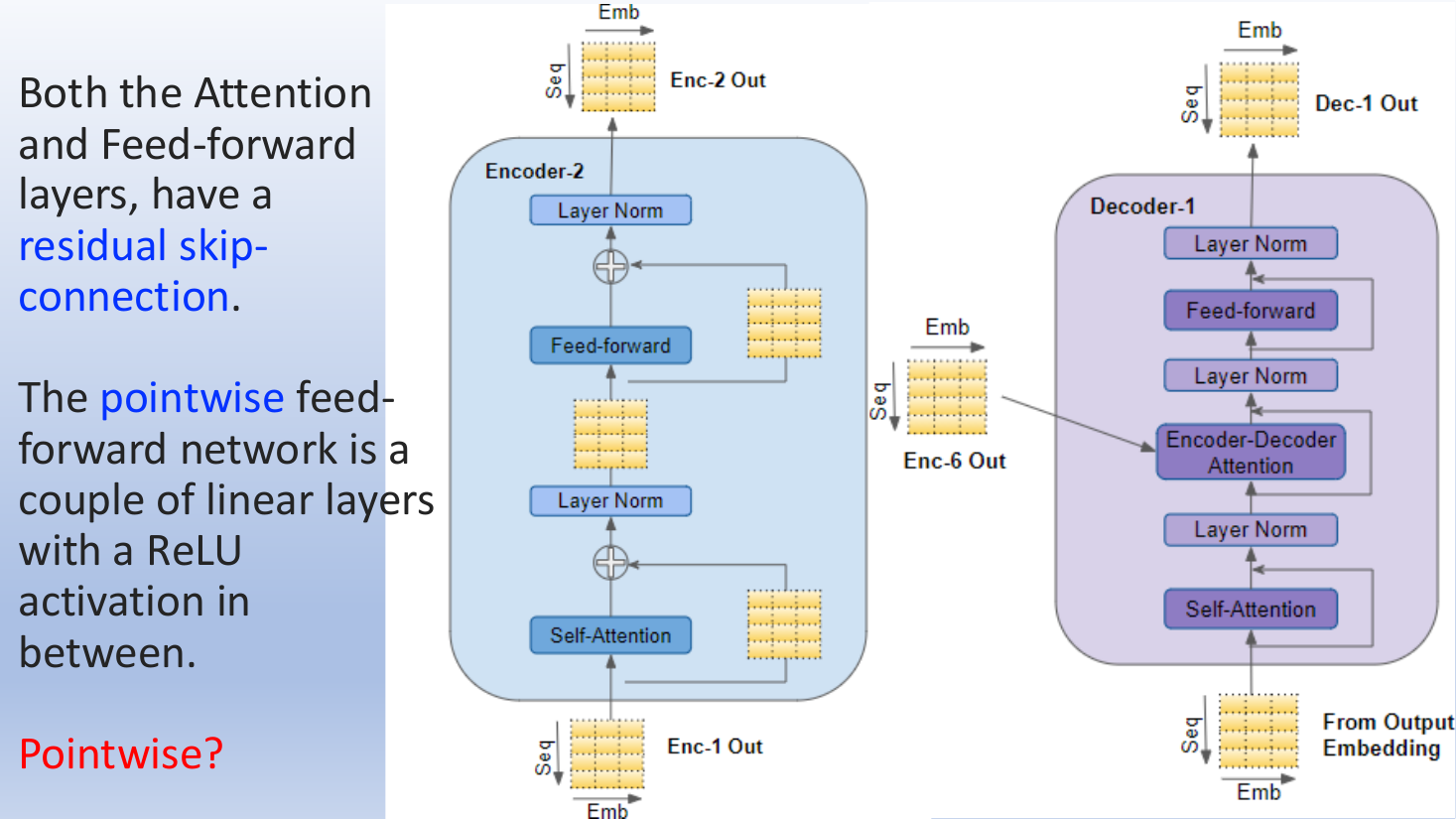
Both the attention layer and the feed-forward layer have a residual skip-connection. Writing a layer as a function applied to its input token matrix :
Explaining each part:
- is the in the figure: the input skips past the layer and is added to the layer's output, so the layer only has to learn a change to its input
- the skip path also lets the error signal pass straight back through a deep stack during training
- layer normalization then shifts and scales each token's features to zero mean and unit variance, followed by a learned scale and shift shared by all tokens, which keeps the numbers in a stable range from layer to layer
- the shapes do not change: input and output are both , so layers can be stacked
The same figure also says the feed-forward network is a couple of linear layers with a ReLU activation in between, and it is pointwise. What "pointwise" means is explained in Pointwise Feed-Forward Network.
Why do we need this
It is the interface between raw data and the network, and it fixes the shape that every layer keeps. The row convention explains the shape of every formula that follows.
Next step
Query Key and Value Projections makes three versions of every token from .
Visual 1: sinusoidal position codes
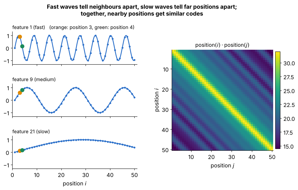
Three of the features of the fixed sine and cosine position vectors, for positions 1 to 50:
- a fast feature changes a lot between positions 3 and 4 (orange and green), so it tells neighbours apart, but it repeats every few positions
- a slow feature hardly changes between 3 and 4, but it keeps changing over many positions, so it tells far positions apart
- together the fast and slow waves give each position its own pattern, a bit like the digits of a number
- right: the dot product of two position vectors is largest on the diagonal and falls as the positions move apart, so nearby positions get similar codes
- this vector is added to the embedding, (Step 3)
Visual 2: word order needs position codes
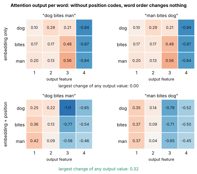
Self-attention outputs for "dog bites man" and "man bites dog", with the rows sorted by word so the same word sits on the same row:
- top: with embeddings only, each word gets exactly the same output in both sentences, so attention cannot tell the two orders apart
- bottom: after adding position the outputs differ, by up to 0.32, because each word now carries where it sits
- the reason is that is a sum, and reordering the terms of a sum does not change it (Step 3)