Introduction
Attention is the core of the Transformer. For each token, it scores how relevant every token is, using a dot product of a query with a key. It then outputs a mix of all the value vectors, weighted by those scores. Every output token therefore carries information from the whole sequence, and the weights are decided by the input itself.
Main idea
Scores $\mathbf{R}=\mathbf{Q}\mathbf{K}^T$ ($N\times N$), where entry $(i,j)$ is $\mathbf{q}_i\cdot\mathbf{k}_j$, the similarity of token $i$'s query with token $j$'s key. Output $\mathbf{Z}=\text{softmax}\left(\mathbf{Q}\mathbf{K}^T/\sqrt{d_k}\right)\mathbf{V}$, or, leaving out the normalization, $\mathbf{z}_i=\sum_j(\mathbf{q}_i\cdot\mathbf{k}_j)\,\mathbf{v}_j$. Each output token is a weighted sum of all value tokens, so it captures global information. The combining weights are computed from each input at run time, so the attention step has no learned weights of its own.
Overview
The sizes, with tokens of features:
Row of holds the weights for output token , one weight per input token .
Step 1: attention scores
The first step of attention is a matrix multiplication (dot products) between the Query matrix and the transpose of the Key matrix:
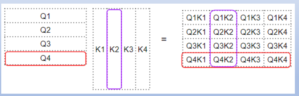
Why entry is :
- row of is , and column of is written as a column
- so entry of the product is row times column , the dot product
- in the figure, the red row meets every column to give the red row of scores, and the purple column meets every row to give the purple column
What the scores mean:
- a dot product is large when the two vectors point the same way, so it measures the similarity (relevance) of the two words
- is an "factor" matrix: one cell for every pair of words
- is not symmetric in general, because uses and while uses and , so how much word attends to word can differ from the reverse, which is also why and have separate weight matrices
- it is a similarity matrix: each entry is the dot product of two tokens, each first mapped by its own learned matrix, so is a learned measure of how related tokens and are; it looks like a covariance (one entry per pair, a sum of products), but nothing is centred or averaged over samples
Step 2: weighted sum of values
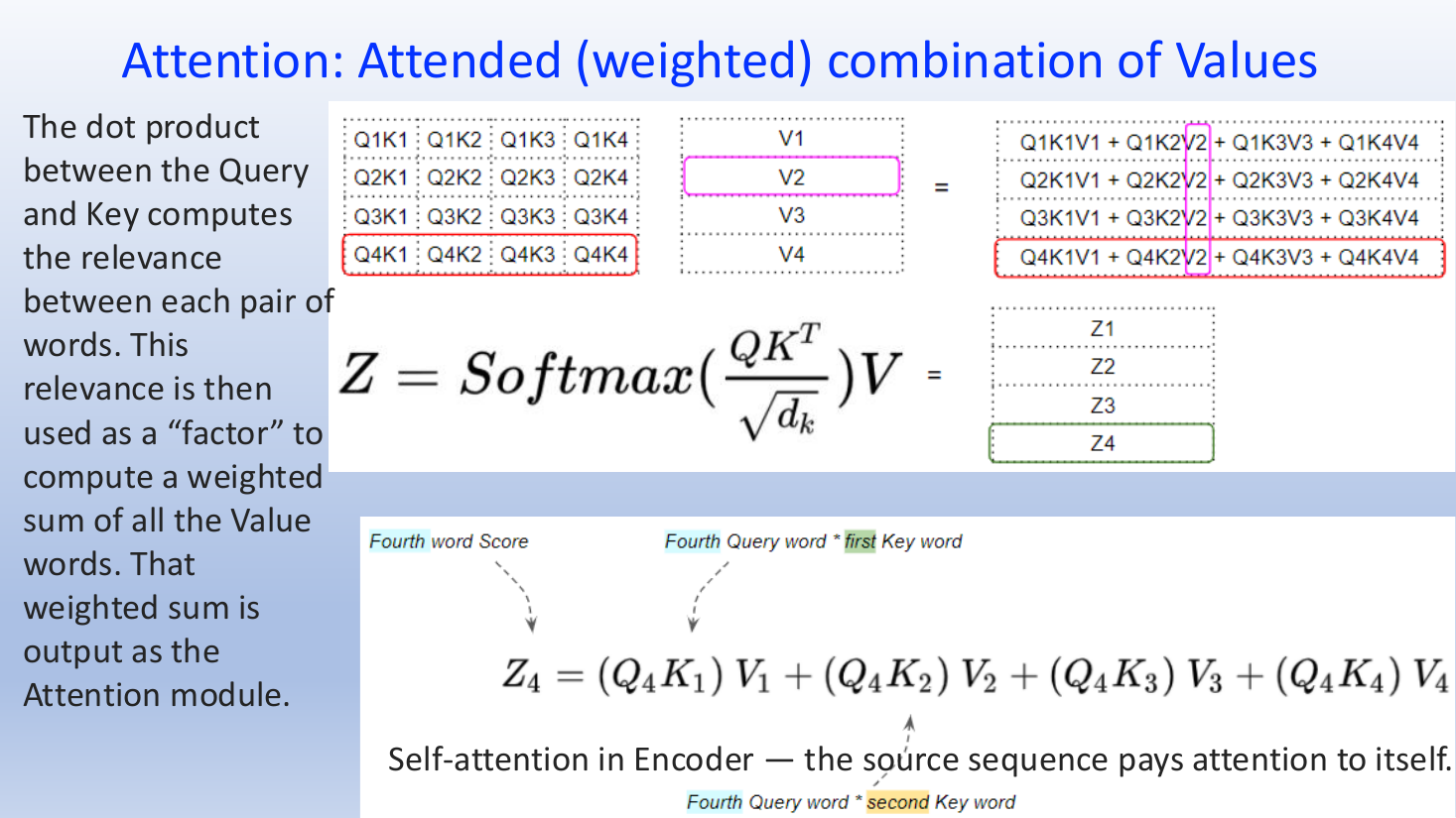
The relevance scores are used as factors to compute a weighted sum of all the value words. That weighted sum is the output of the attention module:
Why row of is this sum: row of a product is , and row of is .
For the fourth word, as in the figure:
The fourth query is matched with every key, and each match decides how much of that word's value goes into . In the encoder this is self-attention: the source sequence pays attention to itself.
Step 3: scaling and softmax
The full attention formula normalizes the scores before using them:
The two extra steps:
- dividing by , where is the length of a key vector (here , or the width of one head when there are several heads), keeps the scores in a stable range
- softmax is applied to each row of scores, turning the scores of one query into positive weights that add up to 1:
Why :
- if the entries of and are independent with zero mean and unit variance, is a sum of such products, so its variance is
- dividing by brings the variance back to 1
- without it, long vectors give very large scores, the softmax then puts almost all the weight on one token, and training gets tiny gradients
What softmax gives: the weights in each row are positive and add up to 1, so each is a weighted average of the value rows.
Masking, used in the decoder's self-attention:
- before the softmax, set for every
- then , so token gives zero weight to all later tokens, which have not been generated yet
Both are a normalization. The structure "weighted sum of values, with weights from query and key similarity" is the same with or without them, which is why the simpler form is used to explain attention.
What softmax means across the topics:
- the Bayes posterior is a softmax of the discriminant scores: with ,
- the Gaussian Parzen window gives each sample a weight that falls with distance, and normalized these weights are a softmax of negative squared distances
- so attention is a weighted average whose weights come from a learned similarity, and dividing by works like the window width : too sharp puts almost all the weight on one token, like the NN rule, and too flat gives a plain average
Step 4: global and not learnable
What the output captures:
- each output token is a weighted sum of all input tokens, so it captures global information from the whole sequence in one step
How attention differs from an MLP and a CNN:
- in an MLP or a CNN, the weights that combine the inputs are learned from the training data and stay fixed afterwards
- in attention, the combining weights are computed flexibly from the specific test input (a new input after training) at run time, so they change with every input
- these weights still depend on the learned and , but they are not stored as fixed numbers
- so the attention step itself is not learnable: the scores and the weighted sum have no weights of their own, and only the linear layers around it (, , and the merge layer after the heads) are learned
Step 5: encoder-decoder attention
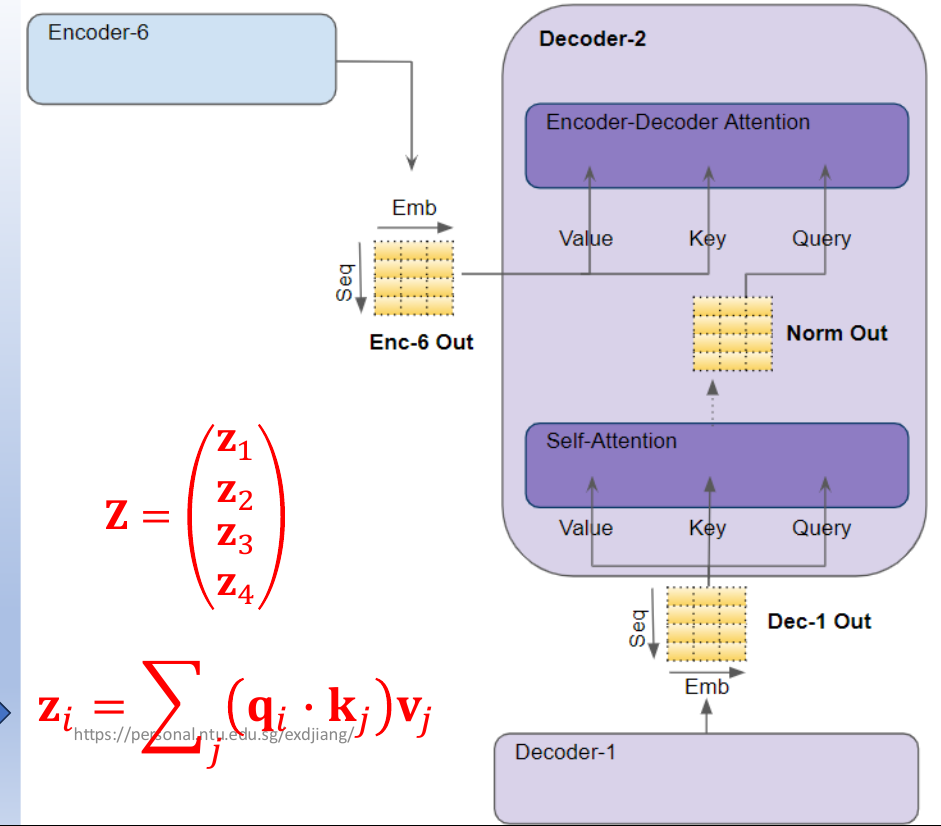
In the decoder's encoder-decoder attention:
- the output of the final encoder in the stack (Enc-6 Out) is passed in to make the keys and values
- the output of the decoder's self-attention module below it (after normalization) is passed in to make the queries
- the same formula then applies, , so
What changes in the sizes: with target tokens and source tokens, is and are . So is : each output word scores every input word, and its output is a weighted sum of the input words' values.
Why do we need this
Attention lets every token gather information from the whole sequence in one step, with weights that adapt to each input. This is what lets a Transformer relate distant tokens directly.
Next step
Pointwise Feed-Forward Network processes each attention output on its own.
Visual 1: following one row of attention
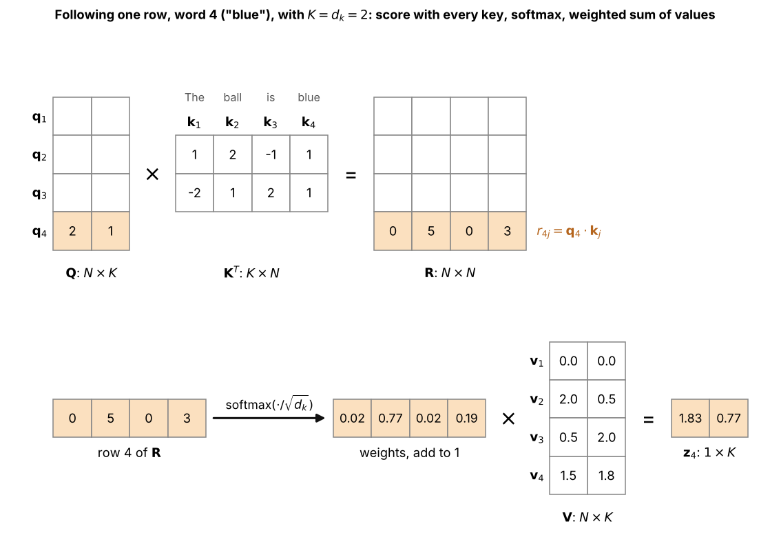
The sentence "The ball is blue" with tokens and features, so , , and all have the same width as the boxed formula says:
- top: the query of word 4, , is dotted with every key, which fills only row 4 of :
- the key of "ball", , points the same way as , so it scores highest (5), and and are at right angles to it, so they score 0
- bottom: dividing by and taking the softmax turns the row into weights that add up to 1, with 0.77 on "ball"
- is then , mostly the value of "ball"
- every other row of and is filled the same way with its own query
Visual 2: output as an average of the values
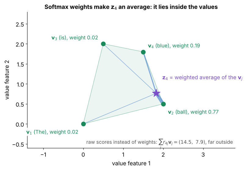
The four value vectors of the example above drawn as points, and as a star:
- is the weighted average of the , using row 4 of the softmax weights
- the line from to each is thicker when its weight is larger, so is pulled mostly toward ("ball")
- the softmax weights are positive and add up to 1, so always lies inside the shaded region spanned by the values
- the simpler form with raw scores, , lands at , far outside, which is what the normalization in Step 3 prevents
Visual 3: why divide by
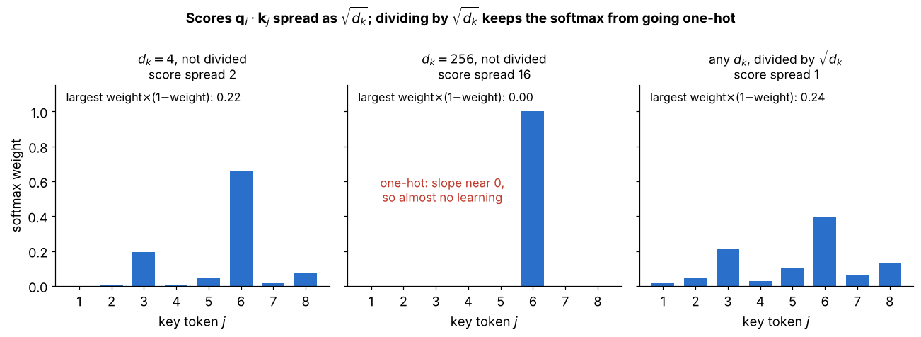
One row of 8 scores with a fixed pattern, stretched by , because a dot product of unit-variance terms has spread :
- left: with the scores spread by 2, and the softmax already leans on one token
- middle: with the scores spread by 16, and the softmax puts all the weight on one token (one-hot)
- right: after dividing by the spread is 1 for every , and the weights stay spread out
- the slope of a softmax weight is weight(1weight), which is near 0 when every weight is 0 or 1, so a one-hot softmax passes back almost no gradient (Step 3)