Introduction
Many functions fit the training data, so learning needs a reason to prefer the one that also fits new data. Regularization gives that reason: it uses human knowledge about the problem to restrict or constrain the learned function . This answers the question "is human knowledge useless?", and a CNN is one of its most successful forms.
Main idea
The training samples alone cannot pick the right $\hat{f}$. Regularization adds human knowledge so that $\hat{f}(\mathbf{x})\Rightarrow f(\mathbf{x})$ for the whole population. It can restrict $\hat{f}$ to a smaller family $\Omega$, require $\hat{f}$ to fit transformed samples $\mathbf{W}\mathbf{x}_i$ and $\mathbf{W}\mathbf{y}_i$, add a penalty $\lambda\Phi(\hat{f})$, or use all of these.
Overview
Every form of regularization changes the plain learning problem in one place:
Step 1: problem to solve
Learning alone only gives on the training samples. The real goal, where means "gets close to", is:
Why the samples alone are not enough:
- the error only checks at the training points
- between those points, many different functions give the same zero error
- so the information that picks the right one must come from outside the samples, from us
Step 2: regularization
Regularization uses human knowledge to restrict or constrain , so that:
The knowledge is about the problem itself, for example how images behave. It is added to the learning problem in one of three ways.
Step 3: three ways to regularize
Start from the plain training error, then change it.
1. Restrict the family of functions. Only search among functions in a set that we believe holds good answers:
What it does: a smaller leaves fewer functions that fit the samples, so the one found is more likely to be close to .
2. Fit transformed samples. Apply a known transform to the inputs and the outputs, and ask to fit the transformed samples. Here is a transform of the samples, not the network weights:
What it does: if we know how the answer should change when the input changes, must follow that rule. For a shifted object the class stays the same, so the transform on leaves it unchanged.
3. Add a penalty. Add a term that grows when is complicated, weighted by :
What it does: sets the balance between fitting the samples and keeping simple. A common choice of is the sum of the squared weights: small weights keep each layer's output a gentle function of its input, so cannot swing sharply between the samples.
For a linear layer fitted by least squares, this penalty adds a constant to the diagonal of , the same fix as adding to a covariance in Eigenvalue Regularization.
4. Or use all of the above.
Step 4: where human knowledge has already been used
Human knowledge restricted in earlier topics too:
- assuming Gaussian classes restricts the class probability densities to one family of shapes, the first form
- reducing dimensions with PCA or LDA before classifying lets use only a few projected features, also the first form
- a CNN only allows small filters whose weights are shared across the image, so it searches a much smaller family than a fully connected MLP
Why do we need this
Regularization is how a network gives up a little fit on the training data for a much better fit on new data. The CNN is the clearest case: its structure is human knowledge about images, and that is why it generalizes where an MLP does not.
Next step
Convolutional Layer shows the restricted structure that a CNN uses.
Visual 1: weight penalty with three values of
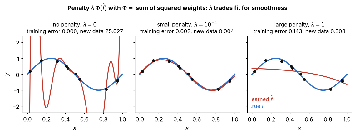
The same 10 samples and 10-weight polynomial as in Generalization Problem of Neural Networks, now fitted by with the sum of the squared weights:
- : the plain training error, which reaches zero, but swings wildly between the samples
- small : the training error rises a little, and the error on new data drops from about 25 to 0.004
- large : the weights are pushed so close to zero that is too flat, which is under-fitting
- so sets the balance between fitting the samples and keeping simple, the third form in Step 3
Visual 2: fitting rotated copies of the samples
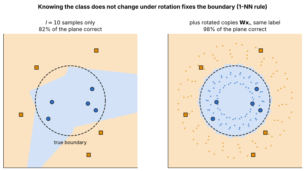
Two classes in the plane, inside the dashed circle (blue) and outside it (orange), classified by the nearest training sample:
- left: with only the 10 samples, the regions follow wherever the few samples happen to lie, and 82% of the plane is correct
- right: we know the class does not change when a point is rotated about the centre, so each is rotated in steps of to give , with the same label
- the boundary now follows the true circle, and 98% of the plane is correct
- this is the second form in Step 3: must fit and , where because the class stays the same