Introduction
A CNN is built from a few kinds of parts, and the convolutional layer is the main one. Instead of joining every input to every output, it slides a small filter across the feature maps and computes a weighted sum at each position. This note lists the parts of a CNN, writes the convolutional layer as a formula, and works out its output size and its number of parameters.
Main idea
$y_{i,j,k}=\sum_{n=1}^{C}\sum_{m=-1}^{1}\sum_{l=-1}^{1}w_{l,m,n,k}\,x_{i-l,j-m,n}+b_k$: output channel $k$ has one filter that covers a $3\times3$ window and *all* $C$ input channels, plus one bias. The weights do not depend on the position $(i,j)$, so the same filter is used everywhere. A layer of $D$ filters of size $F\times F$ on $C$ channels has $D(F^2C+1)$ parameters, whatever the image size.
Overview
One convolutional layer maps a stack of feature maps to another stack:
Each of the output channels comes from its own filter, and each output value uses a window through all input channels.
Two words used everywhere below:
- a feature map is a 2-D array of values, one per image position
- a channel is one feature map in a stack: an RGB image has channels (red, green, blue), and each filter of a layer makes one output channel
Step 1: five parts of a CNN
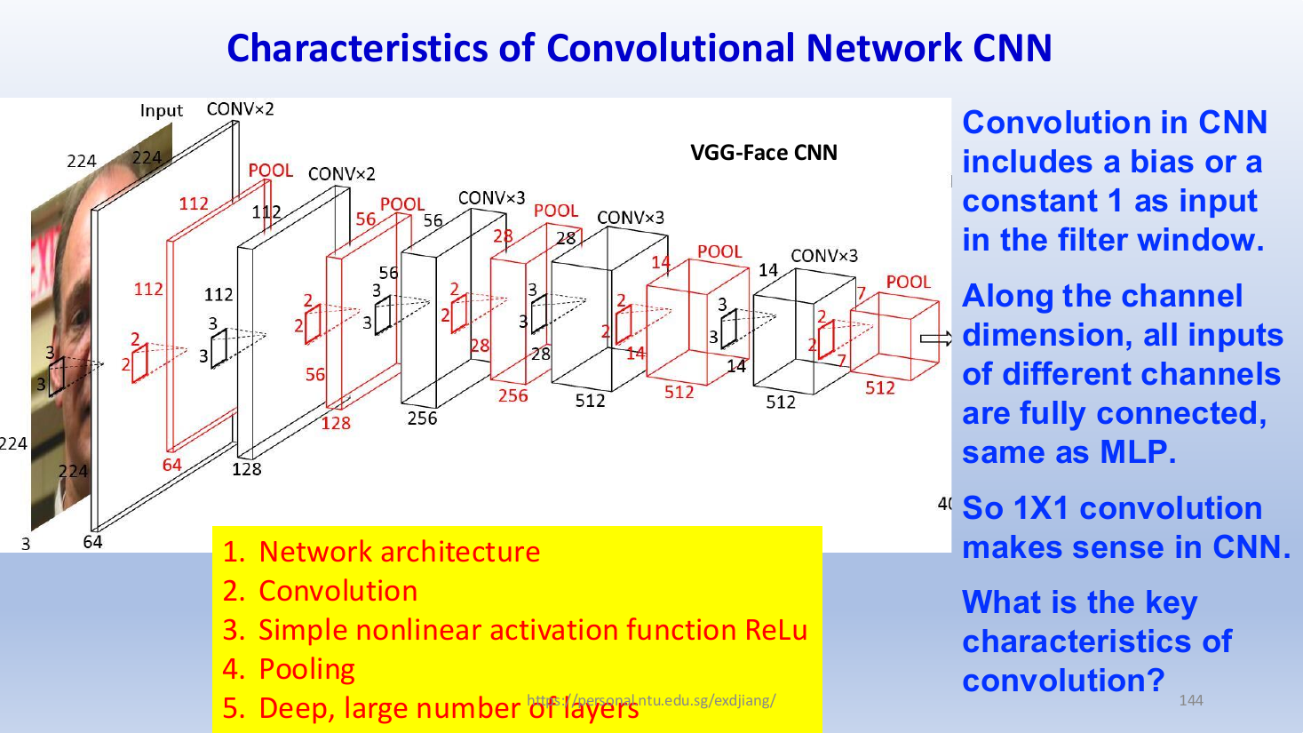
The figure is the VGG-Face network, where each box is a stack of feature maps and the numbers on it are height, width and channel count. A face image goes through blocks of convolutions (CONV×2, CONV×3) with pooling between them, down to , then to fully connected layers. Its five key parts:
- network architecture: the order of blocks and the size of each feature map
- convolution: small filters slid over the feature maps
- simple nonlinear activation function, ReLU: applied after each convolution
- pooling: shrinks the feature maps between blocks ()
- deep: a large number of layers
The ReLU function keeps positive values and sets negative ones to zero:
Together with the bias, it works as a learned threshold: is nonzero only where the filter response is above .
Max pooling replaces each small window of a feature map by its largest value, on each channel on its own. With a window and stride 2 (the step between windows, Step 4), it halves the height and width and has no weights to learn. A small shift of a feature that stays inside the same window does not change the pooled value.
Step 2: what a convolution includes
Three points about convolution in a CNN:
- it includes a bias, which is the same as a constant input of 1 in the filter window, with the bias as its weight
- along the channel dimension, all inputs of the different channels are fully connected to each output, the same as in an MLP
- so a convolution makes sense in a CNN: it looks at no neighbours, but it still mixes all channels at each pixel, like a small MLP applied at every pixel
This leaves the question that the next note answers: what is the key characteristic of convolution?
Step 3: convolution formula
Input feature maps of spatial size with channels, and output feature maps of spatial size with channels, are written as:
Here always counts input channels and always counts output channels.
With filters, weights and biases :
This is the value before the activation. The layer then applies ReLU to every value, , before the next layer.
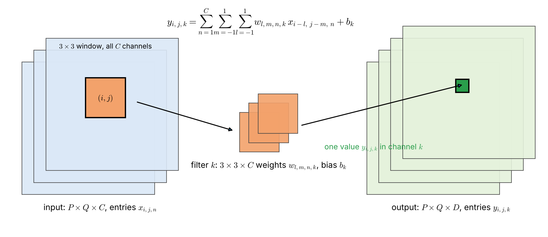
How to read the three sums:
- and run over the window around position , from to in each direction
- runs over all input channels, so one output value uses inputs
- picks the output channel: each output channel has its own filter and its own bias
- the weights have no or in them, so the same filter is used at every position, which is weight sharing
- the output keeps the size when the edges are padded with zeros, so that a window fits around every input position
Turning the filter. The index makes this a true convolution: as goes up, the input index goes down, so the filter is turned by before it is slid. Sliding the filter without turning it (multiply matching entries and add) is called correlation. The two agree when the filter looks the same after a turn. The filters are learned anyway, so a trained network just learns the turned version of the same filter.
Step 4: output size with stride and padding
The stride is the step between two windows, and the padding is the number of rows and columns of zeros added on each side. With an input of size along one side and a filter of size :
Why this formula:
- after padding, the side has values
- the first window starts at position 1, and the last window must still fit, so its start can be at most
- the starts are apart, so there are steps, plus 1 for the first window
With , and , the output size is , which is the same-size case in the formula above.
Where each window sits, written from its top-left corner so that it also works for an even :
What changes from the Step 3 formula:
- the window for output starts inputs after the window for the output before it, so its top-left corner is at
- the filter is laid on the window without turning, which is correlation, the form most CNNs use
- an index outside to falls in the padding and reads as zero
Hint
For one filter on an input with several channels, with a stride:
- a filter of size has one slice per input channel, and gives only one output channel
- each output value is the sum over all channels of (slice times its window), plus the bias
- find the output size from the formula above before computing any value
- before choosing convolution or correlation, check whether a turn changes each slice
- an input written as lists the channels first
Step 5: number of parameters
Each output channel has one filter of weights and one bias. With output channels:
What this shows:
- the count does not depend on or , because the same filter is used at all positions
- a fully connected layer between the same input and output would need weights, one for every input and output pair
- each output value needs multiplications, and there are (output height)(output width) output values
Step 6: what the filters learn
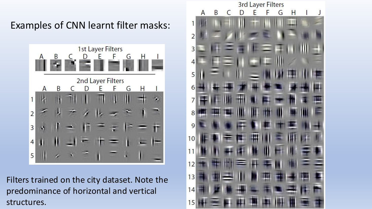
Filters trained on a city dataset are mostly horizontal and vertical structures, the lines of buildings and roads.
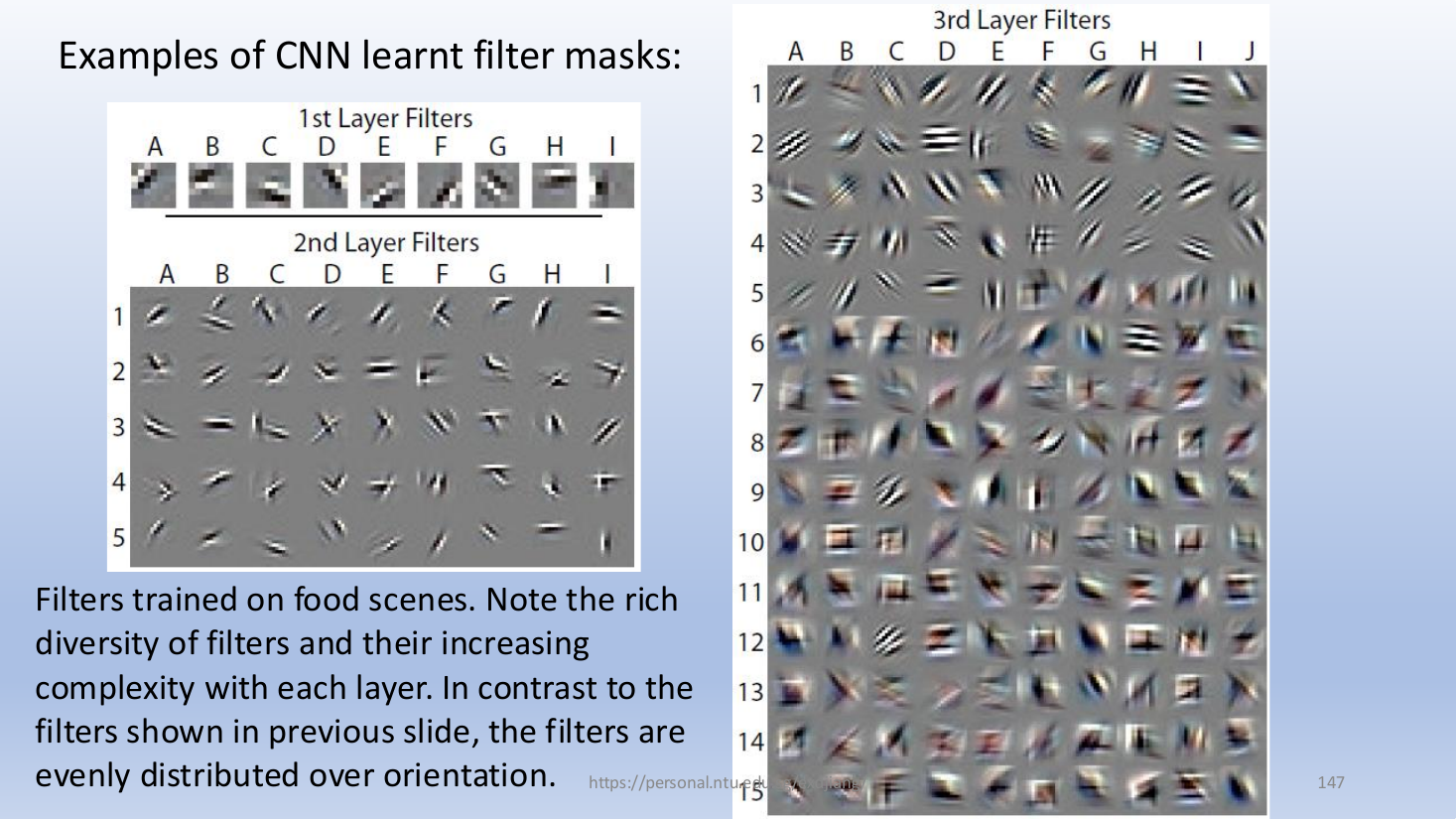
Filters trained on food scenes are much more varied, spread evenly over all orientations. In both cases the filters grow more complex from layer to layer: the first layer finds edges and lines, and later layers combine them into textures and parts.
Why do we need this
The convolutional layer is where a CNN keeps its human knowledge: a local pattern detector that is useful in one place of an image is useful everywhere. It also makes the layer tiny compared with a fully connected one, so many layers can be stacked without a huge number of parameters.
Next step
CNN as a Regularized MLP answers what the key characteristic of convolution is, and why it generalizes.
Visual 1: windows for stride 1 and stride 2
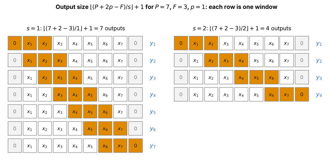
One side of the input, , padded with zero at each end, with a filter of size :
- each row shows, in orange, where the window for one output sits
- with the window moves one place each time, giving 7 outputs, the same size as the input
- with it moves two places, giving outputs
- the last window must still fit inside the padded row, which is why the formula subtracts and then adds 1 (Step 4)
Visual 2: worked convolution with bias and ReLU
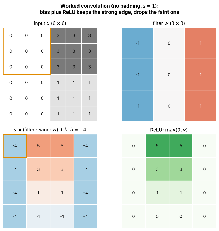
How to read it:
- the input has a strong vertical edge (0 to 3) in the top half and a faint one (0 to 1) in the bottom half
- the filter is laid on each window without turning (correlation), multiplied entry by entry and summed, then is added; the orange boxes are the first window and its output
- windows fully on the strong edge give , windows fully on the faint edge give , flat windows give , and windows that cover both halves give and
- ReLU keeps only values above zero, so is a learned threshold that passes only responses above (Step 1)
- the same 9 weights and 1 bias give all 16 outputs, which is weight sharing
Visual 3: max pooling and small shifts
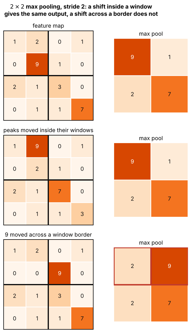
How to read it:
- each black box is one window, and the pooled map keeps the largest value of each window
- middle: both peaks move one pixel but stay inside their windows, so the pooled output is unchanged
- bottom: the 9 moves across a window border into the next window, so two pooled values change (red boxes)
- so pooling ignores small shifts inside a window, not every shift; it also halves the height and width and has no weights to learn (Step 1)