Introduction
Supervised learning tries to find an unknown function from a finite set of examples. An MLP can match those examples perfectly, yet still be wrong almost everywhere else. This note states the learning problem in symbols and shows why fitting the training data is not enough.
Main idea
Learning minimizes the training error $e^2=\sum_i\|\mathbf{y}_i-\hat{f}(\mathbf{x}_i)\|_2^2$. A network with $m=2$ layers can already drive this to zero, but that only gives $\hat{f}(\mathbf{x}_i)=\mathbf{y}_i$ on the $l$ training samples, and $\hat{f}(\mathbf{x})\neq f(\mathbf{x})$ for the rest of the population. Getting stuck before fitting the samples is **under-fitting**. Fitting the samples but not the population is **over-fitting**, and it is the serious problem.
Overview
The note is one chain of four steps:
Step 1: supervised learning
There is an unknown mapping, a continuous function, from an input vector to a class label:
What each symbol is:
- is a sample with real-valued features, such as the pixels of an image
- is the class output with integer entries, written one-hot: the entry of the true class is 1 and the rest are 0, such as for one class and for the other
- is the true rule, which we never see
We only have finite, discrete, known training samples:
Learning looks for an estimate that fits them, by making the total squared error on the training samples as small as possible:
Step 2: neural network solution
A neural network (NN or MLP) builds from layers. Each layer multiplies by a weight matrix and applies a simple nonlinear function :
Reading it from the inside out:
- is a fixed function such as the sigmoid or ReLU, and the bias of each layer is left out to keep the formula short
- counts the weight matrices, so means one hidden layer, a layer between the input and the output
- is the first layer, and turns it into the first hidden layer
- each later layer does the same to the output of the layer before
- the weights are what learning adjusts
- the result is only an estimate , so in general
Step 3: why go deep
In theory, layers are enough to approximate any highly nonlinear function, so the training error can be driven to zero, . This raises the questions behind deep learning:
- if two layers are already enough, what more can be done?
- why did neural networks die out in the 2000s?
- why use deep learning, with layers?
- is the motivation to make the network more powerful, or is the solution easier to find with than with ?
Since two layers are already powerful enough, the answer cannot be more power. The reasons start with the two failure modes below, and for a CNN the full answer comes in the note on CNN as a regularized MLP: depth widens what each output sees, and ReLU keeps the deep layers trainable.
Step 4: under-fitting and over-fitting
Training is an iterative search over the weights that lowers step by step (gradient descent with backpropagation, in the MLP notes). The two problems of learning:
- local minima: the search stops at weights where every small change raises , while is still large, so the network does not fit the training data, which is under-fitting
- poor generalization: training fits the training data but not new data, which is over-fitting
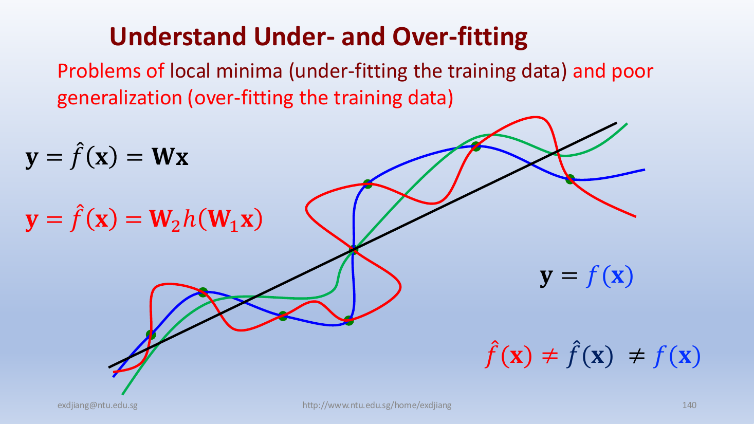
The figure fits the same training points (dots) in three ways:
- , a single linear layer (black line), is too simple and misses most training points, which is under-fitting (here from a model that is too simple, the same symptom as a stuck search)
- , a two-layer network (red curve), passes through every training point but swings wildly between them, which is over-fitting
- the true function (blue curve) also passes through every training point, but takes a different path between them
So means: the red fit, the black fit and the true function all differ. Zero training error does not give , since the red and blue curves agree at every dot and differ almost everywhere between them.
Step 5: problem of machine learning
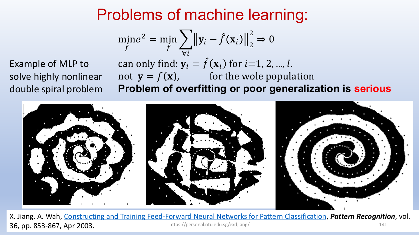
The double spiral problem: each sample is a 2-D point , and the two classes (black and white) are two spirals wound inside each other. The dots are the training samples, and each panel colours every point of the plane by the class the classifier picks. An MLP trained on this highly nonlinear problem shows the problem in full:
What this does and does not give:
- it can only find for , the training samples
- it does not find for the whole population
- the regions learned by the MLP (left two panels) are broken and patchy, far from the clean double spiral (right panel) that a classifier which generalizes well should give
So the problem of over-fitting, or poor generalization, is serious.
Why do we need this
It changes the goal of network design. Making the network more powerful does not help, since two layers are already powerful enough. What helps is making the learned close to on data it has never seen.
Next step
Regularization with Human Knowledge is the general way to do this.
Visual 1: training error against population error
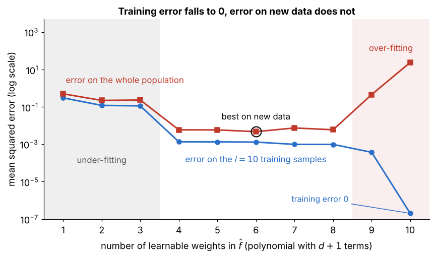
How to read it:
- each point is a polynomial fitted by least squares to the same noisy samples of , with more learnable weights to the right
- the blue training error keeps falling and reaches exactly 0 when has 10 weights, one per sample; a log axis cannot show 0, so that point sits on the floor of the plot
- the red error on the whole population is lowest in the middle and explodes at 10 weights
- left end: too simple, both errors high, which is under-fitting; right end: zero training error but a huge population error, which is over-fitting (Step 4)
- a polynomial is used because it is easy to draw, and a network with more weights than samples behaves the same way
Visual 2: more samples pin down the function
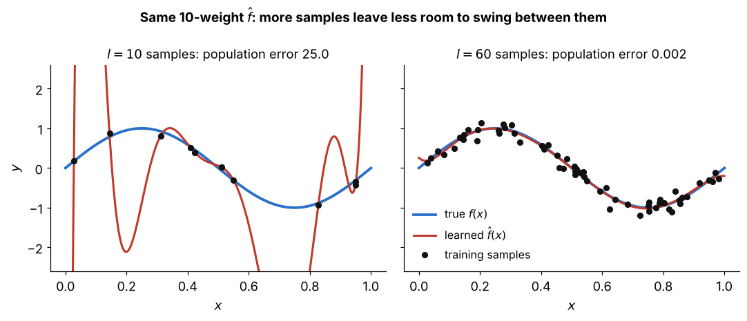
The same model with 10 weights, fitted to two training sets:
- with samples the fit passes through every dot but swings wildly between them, as in Step 4
- with samples there is no room left to swing, and lies on top of
- minimizing only controls at the samples, so more samples per weight means more control between them
- a CNN gets the same effect without new images, by sharing each weight across all pixel positions