Introduction
A convolutional layer can be written as an ordinary MLP layer, , with a very special weight matrix. Comparing the two in 1D shows exactly what a CNN restricts, and why that restriction makes it learn general rules instead of over-fitting. It also answers why CNNs use tiny filters, many layers and ReLU.
Main idea
A CNN is a regularized MLP: its weight matrix $\mathbf{W}$ is mostly zeros, and every row holds the same few filter weights shifted along by one place. So each learnable parameter is used at every input position and is learned from every pixel, which turns one training image into many training samples. Small filters make sure each weight meets every pixel, and deep stacks of them give the large view that one small filter lacks.
Overview
The question this note answers:
The left side is a convolutional layer and the right side is an MLP layer. The answer is yes: the convolution is an MLP layer, with a weight matrix that is restricted in a very particular way. Steps 1 to 3 show this in 1D, and steps 4 to 7 explain what the restriction buys.
Symbols in this note:
- is one input value, and bold is the window of inputs that the filter covers at position
- is one filter weight, bold is the whole filter, and bold is row of the matrix
- is the number of inputs, the filter size, and the number of filters (output channels), which is in the convolution formula
- is the number of training images
Step 1: MLP and CNN in 1D
To avoid distraction, the vector and matrix transposes are left out from here on, so is written .
An MLP layer: output has its own weight for every input :
Here is row of , so is the dot product of row with the whole input. The activation is left out in both layers, because it acts on each output on its own and does not change the weights.
A 1D convolutional layer: every output uses the same small filter , applied to the window of inputs around position :
Reading each equals sign:
- is the 1D version of the convolution formula, with running over the filter, for example
- writes it as the filter times the window , so each meets
- writes the same sum as a full row times the whole input, where the row holds the filter weights at the columns of the window and zeros everywhere else
- stacking the rows gives a matrix , so the convolution is also
Step 2: weight matrix of a convolution
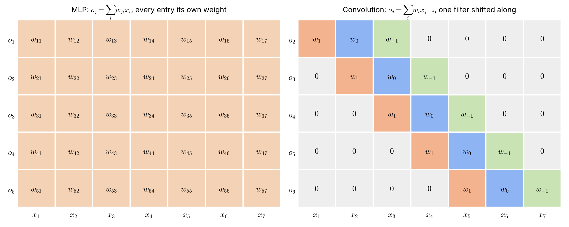
Comparing the two matrices:
- in the MLP (left), every entry is a different weight that has to be learned
- in the convolution (right), row has the filter at columns , and , and zeros elsewhere
- each row is the row above shifted one place to the right, so the whole matrix is a band built from the same three numbers
- the filter appears turned, , because of the in the convolution
- the figure uses no padding, so inputs give only outputs, to , while with zero padding there is one row per input, as Step 4 assumes
Step 3: many filters
A layer has filters , one per output channel. Here is the number of output channels, the of the convolution formula, and not the padding. Each filter gives its own output channel , with a band matrix built from .
Overall shape first: with inputs and outputs per channel, is , made of band blocks of size stacked on top of each other:
So the whole convolutional layer is one MLP layer. Block holds only copies of , and everything outside the bands is zero. Its transpose puts the same blocks side by side.
Step 4: CNN is a regularized MLP
Compare the two weight matrices directly. With inputs, outputs per channel, channels and filters of size :
| Layer | Weights to learn | Each weight is used at |
|---|---|---|
| MLP | , all different | one input position |
| CNN | every input position |
This 1-D count assumes one input channel and no bias. With input channels and a bias it becomes , the 1-D version of .
So a CNN is an MLP whose is restricted: most entries are forced to zero, and the rest are forced to be copies of the same few weights. This is the first form of regularization, searching only a small family of functions. The restriction comes from human knowledge about images: a useful local pattern, such as an edge, is useful at every position.
Step 5: each parameter is learned from all pixels
Step 4 says a CNN searches a much smaller family of functions. This step says why the few weights it keeps are learned well. This is the key characteristic of convolution: the CNN parameter is shared by all input and output pixels.
How a weight learns, from backpropagation: each weight moves along the gradient of the error, and for that gradient is , where is the error signal at output . So a weight learns only from the inputs it multiplies. For a shared filter weight, the gradient adds up over every position, .
What sharing changes for learning:
- in an MLP, weight is only ever multiplied by input , so it learns from one pixel position, and with training images it gets examples
- in a CNN, each filter weight is multiplied by every input position as the filter slides, so with images of positions it gets examples
- this converts one image as a training sample into every pixel as a training sample
- in the terms of the statistical notes, sharing raises the number of training samples per parameter, which attacks the problem of few samples in many dimensions (Rank in Pattern Recognition); overlapping windows are not fully independent samples, but they are many more than one per image
- a rule learned this way has to hold everywhere in the image, so it is a general rule and not a fit to one spot
- this is how a deep CNN overcomes the over-fitting problem and makes the extracted features robust
Step 6: why small filters
A CNN uses the smallest filter sizes, or even .
Why:
- a small filter makes sure each learnable parameter goes through every input point or pixel
- so each parameter learns a general rule over the whole input, and does not over-fit to a specific part of it
- in the extreme, a filter as large as the whole input fits at only one position, so each weight meets only one pixel, which is exactly an MLP
- a small filter has very few weights, each shared by all positions, so every one of them is trained by every pixel and none is spent on one particular place
Step 7: why deep, and why ReLU
Why many layers. One filter only sees a tiny patch, so a CNN needs many layers to capture information from a large area.
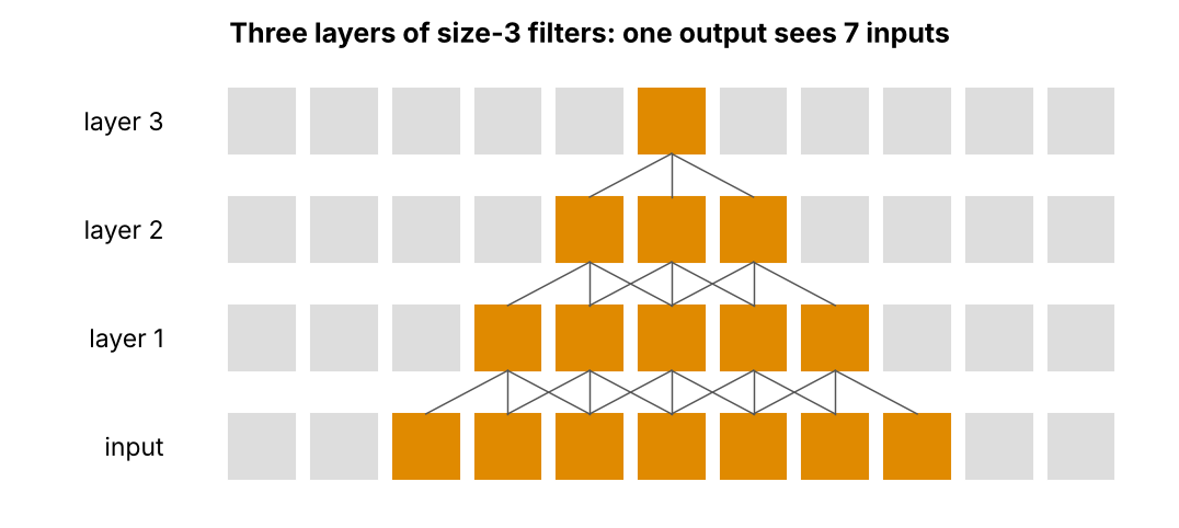
How the view grows with depth:
- each layer of size- filters widens the view by inputs
- after layers, one output depends on a row of inputs along each axis, which is for
- pooling between blocks halves the map, so every later layer covers twice the distance in the original image
Why ReLU. The simplest activation function, ReLU, makes the learning of deep layers easier:
- backpropagation passes the error back through every layer, and at each layer it is multiplied by the slope of the activation function
- for ReLU, for every and for , so on the active units the error signal keeps its size through many layers
- for the sigmoid , the slope is at most , so after layers the error signal is scaled by at most , and the layers near the input barely learn
Step 8: local or global
Does a CNN beat an MLP because the CNN is local while the MLP is global? No. Global information is also learned, by the higher layers of a CNN, whose view covers the whole image after many layers and poolings. The real difference is how the weights are learned: few, shared, and trained by every pixel.
Why do we need this
It explains the design of every modern CNN with one idea, regularization by weight sharing. The same idea returns in the Transformer, whose learnable parts are also shared across all positions.
Next step
Further Development of CNN shows how CNNs are extended to label every pixel of a scene.
Visual 1: how many pixels one shared weight meets
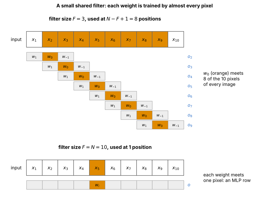
One input row of values, no padding, with the filter written as in the weight matrix of Step 2:
- top: a size filter fits at positions, one per output , and the same weight (orange) is used at every one of them
- the orange input pixels are all the pixels multiplies, 8 of the 10, so it is trained by almost every pixel of every image
- bottom: a filter as large as the input fits at only one position, so each weight meets a single pixel, which is exactly a row of an MLP (Step 6)
- with images, a small filter gives each weight about examples, and the full-size filter only (Step 5)
Visual 2: ReLU against sigmoid in backpropagation
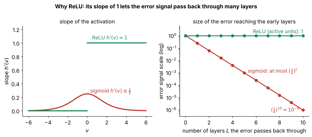
How to read it:
- left: the sigmoid slope peaks at , while the ReLU slope is 1 for every
- right: the error signal is multiplied by one slope per layer, so after sigmoid layers its size is at most times the start
- after 10 sigmoid layers the error reaching the first layer is about of its size, so those layers barely learn
- on active ReLU units the error keeps its size through every layer, which is why deep CNNs use ReLU (Step 7)