Introduction
A basic CNN gives one label per image. Scene segmentation, or pixel-wise scene understanding, asks for a label at every pixel: road, car, person, sky. This note covers three extensions of the CNN for this task: context contrasted local features, gated multi-scale aggregation, and shape variant convolution.
Main idea
To label one pixel well, a network needs the local detail at that pixel and the context around it. Context contrasted local features subtract the context from the local features, $\mathcal{CL}=\mathcal{F}_l(\mathbb{F},\Theta_l)-\mathcal{F}_c(\mathbb{F},\Theta_c)$. A gated sum mixes the scales with learned weights per pixel, $\bar{\mathbb{S}}_p^c=\sum_nG_p^n\,\mathbb{S}_p^{c,n}$. Shape variant convolution lets the context region follow the shape of the object instead of a fixed window.
Overview
All three extensions answer the same question in different ways: which surrounding information should count when labelling pixel ?
| Extension | What it decides |
|---|---|
| context contrasted local features | how a pixel differs from its surroundings |
| gated multi-scale aggregation | how much to trust each scale, at each pixel |
| shape variant convolution | which surrounding pixels belong to the same object |
Step 1: scene segmentation network
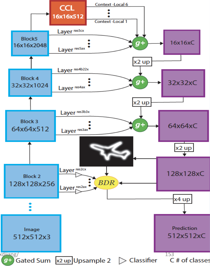
The network takes an image and outputs, at the same size, a score for each class at each pixel (the pixel gets the class with the highest score). A few words used below:
- the backbone is an ordinary CNN whose blocks shrink the feature maps
- a skip layer sends the feature maps of one block straight to the output side
- to upsample by 2 is to double the height and width of a map
How the sizes change, with the number of classes:
- the backbone shrinks a image through blocks of , , and
- a CCL module on the last block gives context contrasted features (Step 2)
- at the last three blocks a gated sum (Step 3) fuses the skip layers into a score map, , then , then , each time adding the upsampled map from the coarser block
- the map is upsampled to , refined near object boundaries with the block 2 features (BDR), and a final upsample gives the prediction
Step 2: context contrasted local features
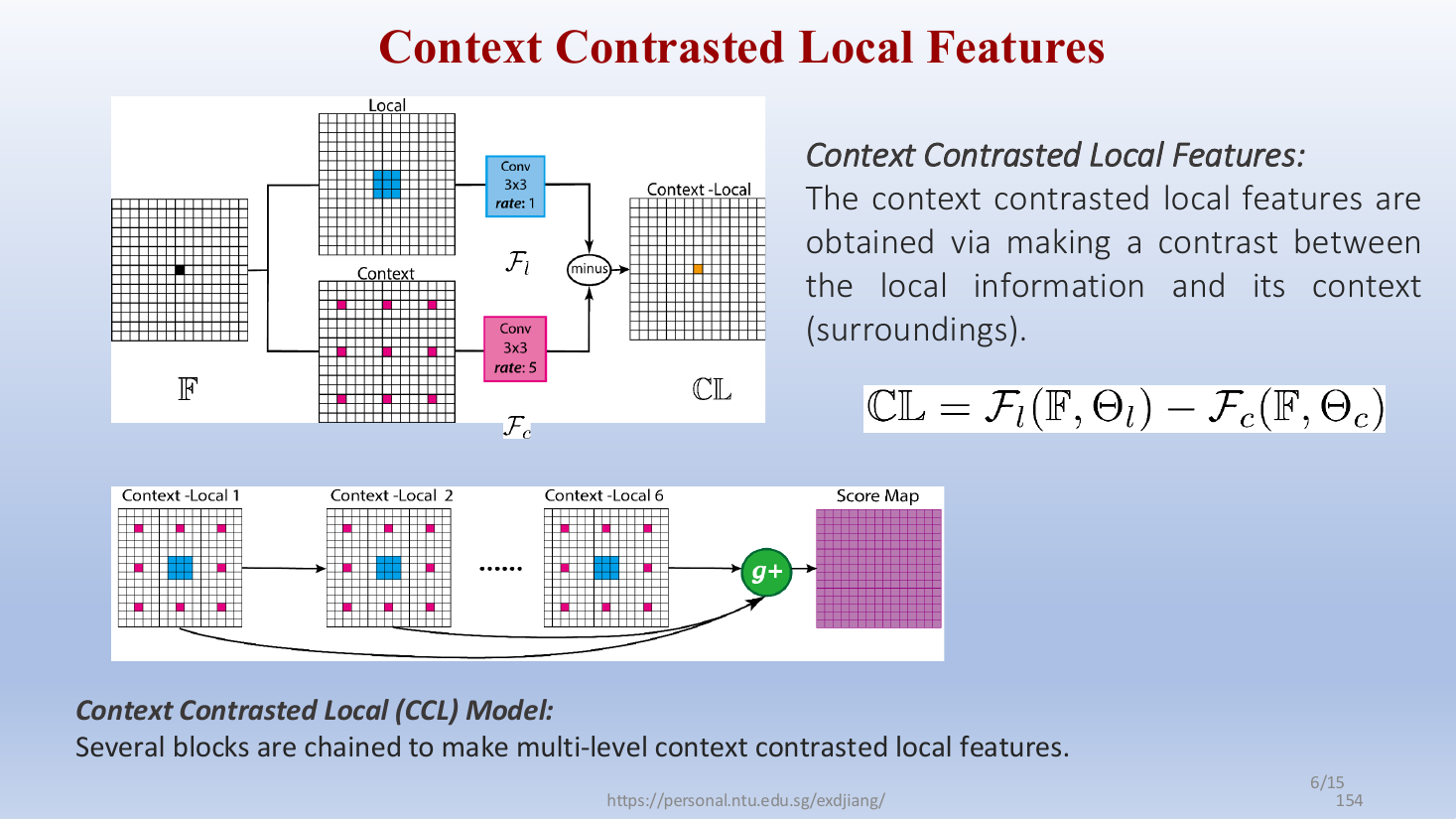
From a feature map , two convolutions run side by side, with weights and :
- a local convolution , a convolution with rate 1, which sees the pixel and its close neighbours
- a context convolution , a convolution with rate 5, whose 9 taps are spread 5 pixels apart, so it sees the wider surroundings with the same number of weights
The context contrasted local features are the difference of the two:
What this does:
- the subtraction removes what the pixel has in common with its surroundings, as seen by the two learned convolutions
- what remains is how the local information differs from its context, so small or inconspicuous objects stand out from a dominant background
- the context contrasted local (CCL) model chains several such blocks, to get context contrasted local features at multiple levels, and fuses their outputs into one score map with a gated sum (Step 3)
Step 3: gated multi-scale aggregation
Each skip layer , from the deepest (coarsest) to the shallowest (finest), gives features at pixel , and a classifier turns them into a score for class . The gated sum fuses the scores with gates that are learned and differ from pixel to pixel:
How to read it:
- is the pixel, is the class, and is the scale (skip layer)
- the gate is how much scale is trusted at pixel
- the gates are computed by the network from the features themselves (the units in the figure), so they change from image to image
- at a pixel inside a large object the network can trust the coarse scales, and at a pixel on a thin object or an edge it can trust the fine scales
- so the outputs of the skip layers are selectively fused, which works better than adding all scales with fixed weights
Step 4: shape variant convolution
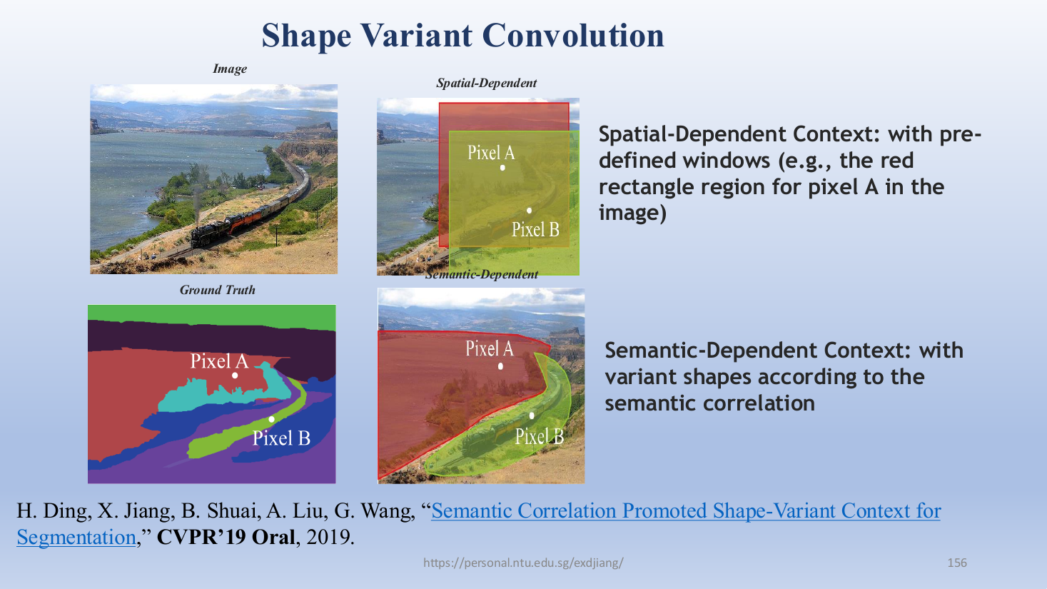
Two kinds of context for a pixel:
- spatial-dependent context uses a pre-defined window around the pixel, such as a fixed rectangle
- semantic-dependent context uses a region whose shape varies with the semantic correlation, so it follows the object that the pixel belongs to
Here semantic correlation means how likely two pixels are to belong to the same object or class.
How shape variant convolution works, for a feature map of size (here is a number of channels):
- a small network (a paired convolution followed by a function ) turns into values at each pixel, which are reshaped into one shape mask per pixel, so masks in total
- each mask gives every position in the window a weight, by how strongly it is semantically correlated with the centre pixel
- the shape variant convolution (SV Conv) multiplies its window by the pixel's own mask before summing, and gives a new feature map of size (here is a number of channels, not a filter size)
- pixels from other objects inside the window get a small weight, so they are suppressed
So the shape variant context aggregates surrounding information according to the semantic correlation, and customizes an effective context region for each pixel. It controls the information flow within the network, by deciding what information is passed and what is suppressed. In examples, the shape masks follow the outline of the object that each pixel belongs to, such as a car or a train. The coloured regions in the figure show the idea of an object-shaped context; the mask itself works inside each window.
Why do we need this
These extensions adapt the CNN to a harder task while keeping its core idea of shared, learned filters. They also point toward the next step: letting the region a pixel looks at depend on the input itself.
Next step
From CNN to Transformer takes that step, with attention.
Visual 1: context contrasted local features on a toy map
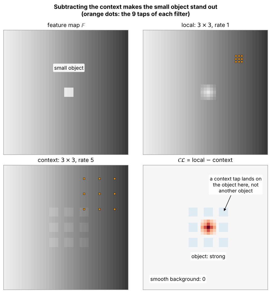
A feature map with a smooth background (bright left, dark right) and one small object a little brighter than its surroundings:
- local: a average with rate 1, whose 9 taps (orange) sit next to each other
- context: a average with rate 5, whose taps are 5 pixels apart, so it sees the wider surroundings with the same 9 weights
- , local minus context, is 0 on the smooth background and strong at the object, so the object stands out even though it is faint in
- the 8 pale squares around the object are not other objects: they are pixels whose spread context taps land on the object
- here both filters are plain averages to show the idea, while in the network and are learned (Step 2)
Visual 2: gated sum along one row of pixels
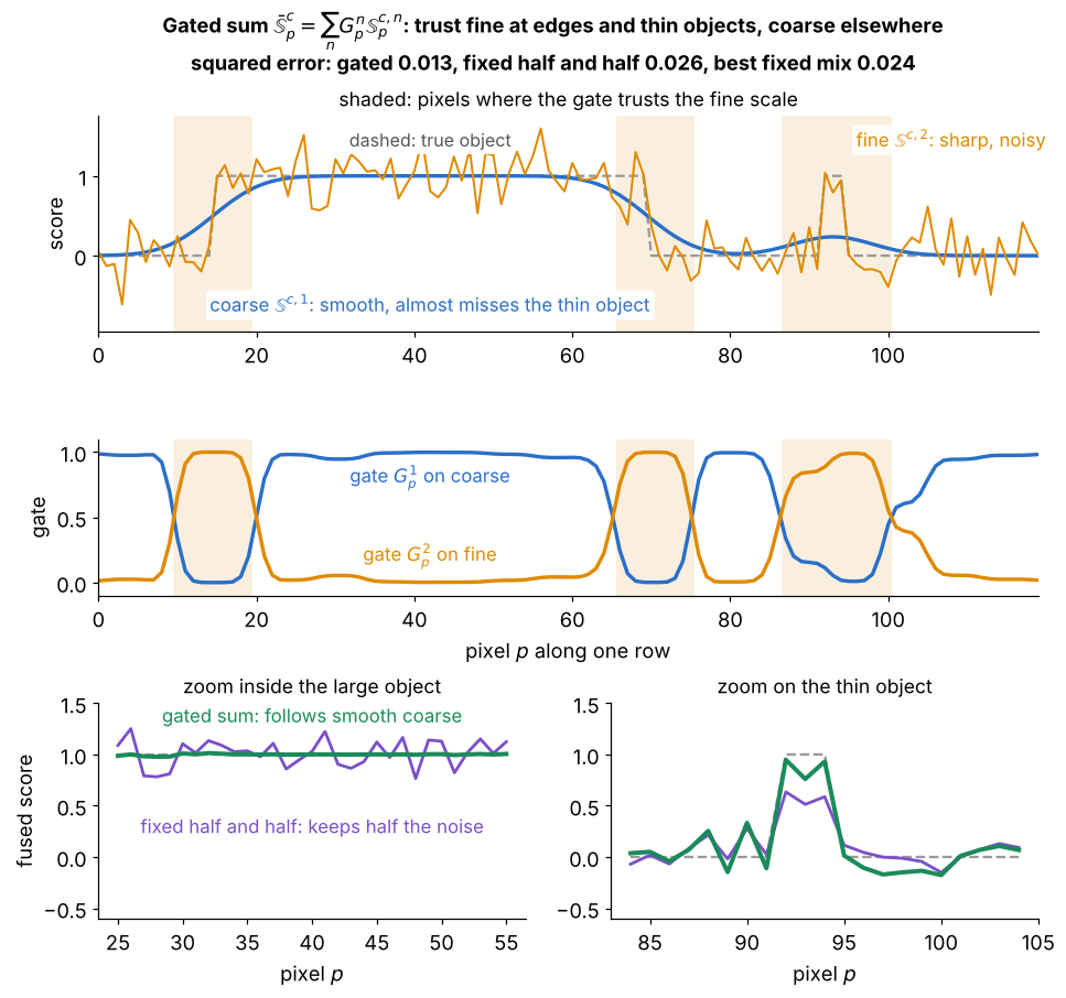
One class , along one row of pixels, with two scales:
- top: the coarse score is smooth but blurs the edges and almost misses the thin object near , while the fine score is sharp but noisy
- middle: the gates trust the fine scale only near the two edges and the thin object (shaded), and the coarse scale everywhere else, with at each pixel
- here the gates come from a fixed rule (how strongly the fine score changes nearby) to show the idea, while in the network they are learned
- bottom: inside the large object the gated sum follows the smooth coarse score, and on the thin object it follows the fine score, while a fixed half and half mix keeps half the noise and half the miss
- so the gated sum, , beats every fixed weighting: squared error 0.013 against 0.024 for the best fixed mix (Step 3)