Introduction
The small eigenvalues learned from training data are much smaller than the true variances of the population, so they give huge, misleading weights in the discriminant function. Eigenvalue regularization keeps all dimensions but replaces the unreliable small eigenvalues with larger values. This note covers solutions 1 to 3.
Main idea
Solution 1 adds a constant $a$ to every eigenvalue. Solution 2 keeps the $m$ largest eigenvalues and replaces the rest with their average $\rho_{av}$. Solution 3 replaces them with the larger $\rho_{up}=\lambda_{m+1}$, because the goal is to match the population variances, which are larger than the training eigenvalues in the tail.
Overview
All three solutions only change the denominators , and each one makes the small ones larger:
Step 1: add a small constant
A common practice in classification and data regression is to regularize the covariance matrix by adding a constant to its diagonal:
Where it comes from:
- it was first used to avoid a singular and the numerical instability of its inverse
- many algorithms for classification, data regression, dimensionality reduction and manifold learning use this classical technique
Why it raises the accuracy. Since , the identity can be written with the same eigenvectors:
So has the same eigenvectors, and every eigenvalue becomes . By the derivation in Discriminant Function in Eigenspace:
What this does:
- a large barely changes, because is small next to it, so the reliable dimensions keep their weights
- a small grows a lot compared with its size, so the weight of an unreliable dimension can never exceed
- the principle is the same as the solutions below: make the small eigenvalues larger
- is chosen by the user, and no rule for it is given here
What adding means physically:
- it is the covariance you get if every training sample is blurred into a small round cloud of variance
- every axis gains spread , so the small eigenvalues are lifted the most in relative terms, and none can stay zero
- the same idea appears as the Gaussian Parzen kernel, which spreads each sample by , and as the squared-weight penalty in Regularization with Human Knowledge, which adds a constant to the diagonal of in least squares
Step 2: probabilistic subspace learning
This solution splits the discriminant function into two parts. It keeps the largest eigenvalues and replaces every smaller eigenvalue with one constant:
The constant is the average of the replaced eigenvalues:
Why the average: it is the best single number to stand for in the least squares sense. Minimize by setting the derivative to zero:
Why one constant also helps in practice: because is orthonormal, , so the second sum equals and the unreliable eigenvectors are never needed.
The number of kept eigenvalues is chosen by the user, and no rule for it is given here.
This solution leads to the Bayesian algorithm, one of the best performers in face recognition.
What the leftover term means: is the squared distance from to the -dimensional subspace of class , which is exactly the PCA reconstruction error of (PCA Reconstruction). So this classifier adds the distance inside the reliable subspace, axis by axis, and the distance from the subspace, weighted by one constant.
Step 3: enhanced probabilistic subspace learning
The key point: the purpose of regularization is not to approximate the training eigenspectrum well. It is to approximate the population variances, which in the tail are larger than the training eigenvalues. So this solution uses a larger constant:
Why is better than :
- every training eigenvalue in the tail is too small, so the best guess of the true variance is the largest one, , not their average
- for the same , , so the weight of the unreliable dimensions is smaller
- the true variances also fall slowly with , so at the far end can be a little too large, but it is still much closer to them than the training eigenvalues
- also continues the weight curve smoothly from dimension , with no jump
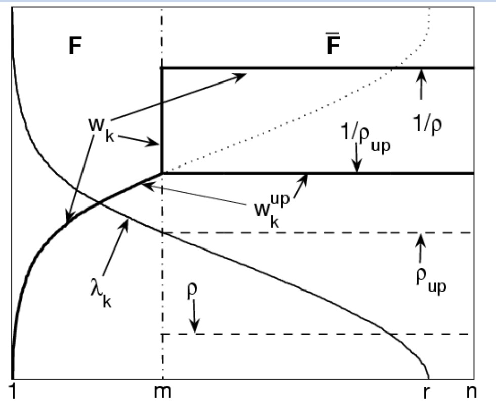
Reading the figure (no scale is given, only the shapes):
- is the decreasing eigenspectrum, with splitting the principal space from its complement , and the number of nonzero eigenvalues
- is the weight of each dimension: the thick curve in , and the dotted curve in , which shoots up as goes to zero
- (upper dashed line) is the value of at , so the weight line (labelled ) starts exactly where is at , with no jump, and it is below every raw weight in
- a smaller constant (lower dashed line), such as , gives the higher weight line to all the unreliable dimensions
Recognition rate (%) of face images against the number of training images:
| Method | 500 | 1000 | 1400 |
|---|---|---|---|
| 89.76 | 90.44 | 89.70 | |
| 91.03 | 93.03 | 93.64 | |
| in | 92.90 | 95.94 | 96.46 |
What the table shows:
- beats for every training size
- the last row applies only inside the -dimensional space of the nonzero eigenvalues, which also removes the null space (the directions where the training eigenvalue is exactly zero), and it is the best
- this last row already mixes regularization with dimensionality reduction, the idea of the next note
Why do we need this
These solutions fix the misleading weights without throwing any dimension away. Solution 3 also shows the right goal for any fix: match the variances of new data, not the training eigenvalues.
Next step
PCA for Classification goes one step further and drops the unreliable dimensions completely.
Visual 1: what adding does
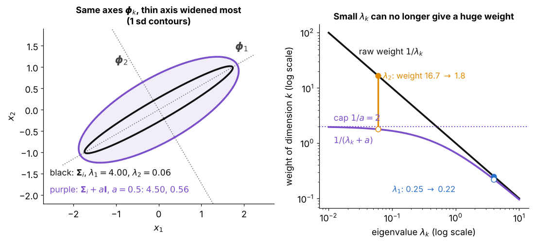
Solution 1 in a picture, how to read it:
- left: keeps the same eigenvectors and only adds to each eigenvalue
- the thin axis grows from to , almost ten times, while the long axis only goes from 4 to 4.5
- right: the weight of the thin axis drops from to , while the weight of the long axis barely moves (0.25 to 0.22)
- however small gets, stays below the cap , which is the point of Step 1
Visual 2: against
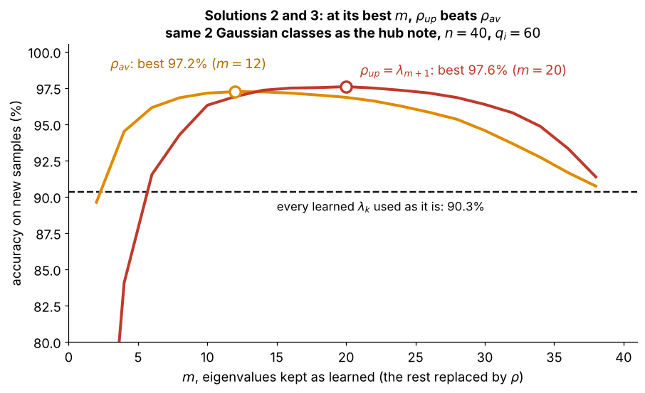
Solutions 2 and 3 on the same simulation as the hub note, how to read it:
- two Gaussian classes, , , accuracy measured on new samples
- the first eigenvalues are kept as learned and the rest are replaced by one constant, (orange) or (red)
- both lift the accuracy from 90.3% to about 97% without dropping any dimension
- at its best , is highest (97.6% against 97.2%), as in the table of Step 3
- for small the order flips, because is then still a large eigenvalue, so gives the many replaced dimensions too small a weight