Introduction
Solutions 2 and 3 replace all the unreliable eigenvalues with one constant. The eigenspectrum model of the eigenfeature regularization and extraction (ERE) method replaces them with a smooth curve instead, so the weights change gradually from the reliable dimensions to the unreliable ones. It is solution 5, and it is applied to the eigenvalues of the within-class scatter matrix .
Here the matrix is the within-class scatter (Scatter Matrices) instead of one class covariance . In face recognition there are many classes with only a few samples each, so all classes share one pooled covariance , and every uses its eigenvalues . The problem of small eigenvalues is the same. The "extraction" part of the method, which picks features after the regularization, is not covered here.
Main idea
Keep the reliable eigenvalues for $k
Overview
The eigenspectrum is split into three regions by two indices, and (the number of nonzero eigenvalues):
Step 1: the model
Here the reliable region is (earlier notes kept ), only a different way to count the boundary.
What each region is:
- () is the reliable region, where the real training eigenvalues are close to the population variances, so they are kept
- () is the noise region, where the training eigenvalues are too small, so the model replaces them
- () is the null space, where the training eigenvalues are exactly zero, so the model value at is used as a constant
One reason for a curve of the form :
- the reliable part of a real eigenspectrum falls off roughly like
- the noisy part falls much faster, toward zero
- extending the shape of the reliable part into the noise region gives a better guess of the population variances than the noisy values themselves
Step 2: fitting the constants
and are chosen so that the model matches the reliable part of the eigenspectrum, and and come from the data and the user.
Extra detail
One simple way to fit and is to make the model pass through the first and the th eigenvalues, and . Solving these two equations:
How the solve goes:
- divide the two equations: , which is linear in and gives
- put back into to get
Step 3: reading the figure
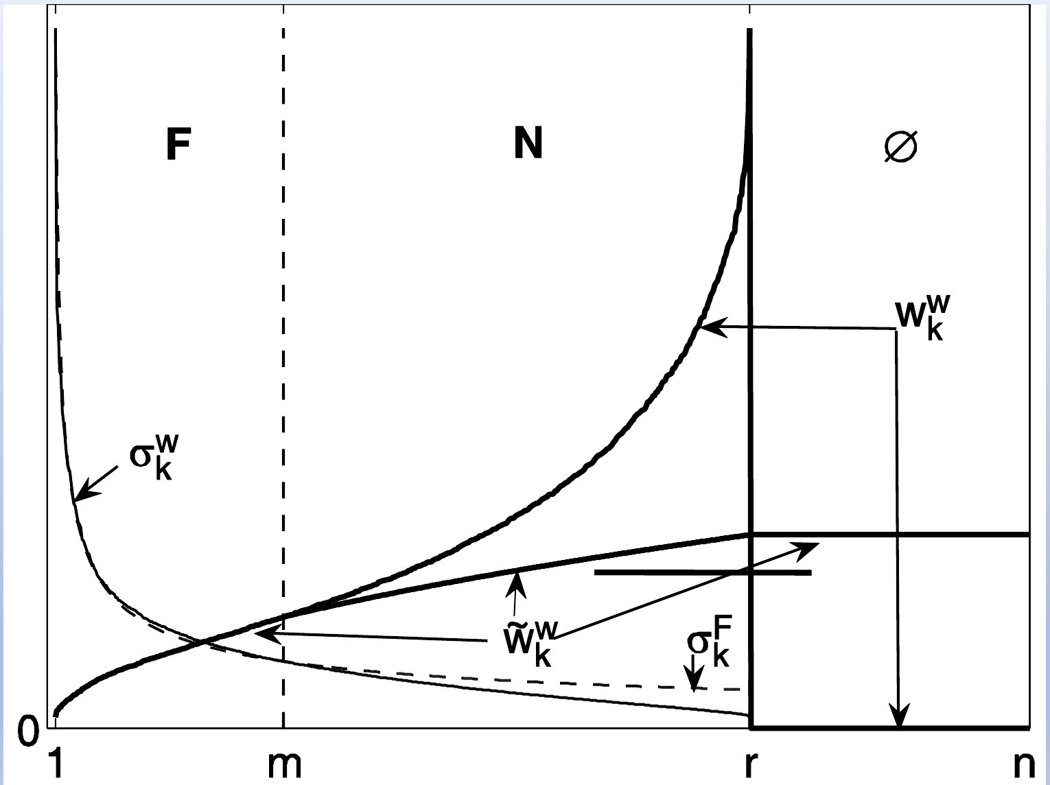
Reading the figure:
- is the real eigenspectrum (the same as ), and the dashed curve is the model , which decays slowly instead of falling to zero
- the real weights shoot up as approaches , and in the null space does not exist, so these dimensions are thrown away, which the figure draws as weight
- the regularized weights grow smoothly through and stay constant in , so no dimension gets an extreme weight
Compared with the earlier solutions:
- solutions 2 and 3 use one flat value for every , so the weight jumps or stays flat
- the model keeps the order of the eigenvalues, so a dimension with a smaller training eigenvalue still gets a slightly larger weight, but never an exploding one
Why do we need this
It gives a closer guess of the population variances in the noise region than any single constant, and it lets all dimensions, including the null space, be used with sensible weights.
Next step
Supervised and Asymmetric PCA changes how the classes are mixed before PCA, so the less reliable class gets more attention.
Visual 1: model fitted to a simulated spectrum
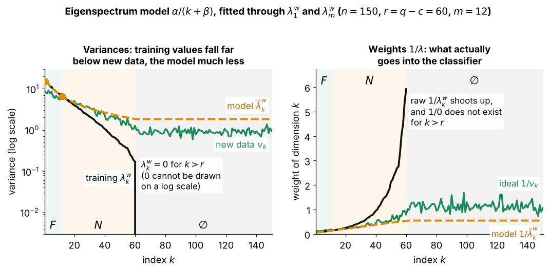
How to read it:
- left: black is the eigenvalues of from samples in classes, so only are nonzero and the rest are exactly 0
- green is , the variance of new samples along the same eigenvectors, the value each should have had
- dashed orange is the model, fitted only through and with (Step 2), and in and it stays far closer to green than the training values
- the simulated variances do not have the form , so the fit is not exact: in the model is about twice the true variance
- right: the weights that enter , where the raw weights explode near and do not exist beyond it, while the model weights stay moderate