Introduction
The MAP rule needs the posterior of every class. It is hard to get directly, but two other quantities are easy: the prior and the class-conditional probability , also called the likelihood. Bayes formula builds the posterior from them. This note derives it from three basic rules of probability, then shows what the MAP rule needs in practice.
Main idea
$p(\omega_i|x)=\dfrac{p(\omega_i)\,p(x|\omega_i)}{p(x)}$ with $p(x)=\sum_{i=1}^{c}p(x|\omega_i)\,p(\omega_i)$. $p(x)$ is the same for every class, so to decide you only compare $p(\omega_i)\,p(x|\omega_i)$. For two classes, the decision changes where $p(\omega_1)\,p(x|\omega_1)=p(\omega_2)\,p(x|\omega_2)$. To decide at every $x$ you need $p(x|\omega_i)$ for all values of $x$, which is the big practical challenge.
Overview
The three probabilities and how they join:
Steps 1 to 4 derive this formula, step 5 uses it to decide, and step 6 shows what it needs.
Step 1: why not the posterior directly
The three probabilities, in words:
- prior : how common class is, the share of the class in the population, before anything is measured
- class-conditional probability : how the measurement is spread inside class only, which you get by measuring many objects of that one class, and it is called the likelihood because, for the measured , it says how likely that measurement is under each class
- posterior : how likely class is among only the objects with measurement
The prior and the class-conditional probability can be measured one class at a time. The posterior needs every class mixed together in its true proportions, with enough objects at every single value of , so it is not straightforward to get. We want a formula for the posterior in terms of the other two.
Step 2: three rules of probability
Conditional probability. Knowing that event happened makes the new whole space. Among the outcomes in , it asks what share also has :
Picture each event as a region inside the whole space , with probability equal to its area divided by the area of . Then is the share of the area of that also covers.
Chain rule (product rule). Rearranging gives the joint probability, and it can be split in either order:
In general . The product form holds only when knowing does not change the chance of , , and then and are called independent.
Law of total probability. If the events do not overlap and together cover everything, then splits into the parts inside each :
The second form uses the chain rule on each part. In the region picture, the regions cut into pieces, and the area of is the sum of the areas of its pieces.
Step 3: Bayes formula
Apply the chain rule to the measurement and the class , splitting the joint probability both ways:
Divide both sides by :
Why the prior and the likelihood are multiplied: the share of all objects that are from class and have measurement is the share of class , times the share of that class that lands at .
For a continuous , such as a height, the chance of one exact value is zero, so the rules for events are applied to the event " lies in a small interval of width ". Its probability is about , where is now a density. The appears above and below the line and cancels, so the same formula holds with densities. These notes write lowercase for both probabilities and densities, and figures that write the prior as capital mean the same thing.
Step 4: mixture p(x)
The classes do not overlap and cover every object, so they are the of the law of total probability. With as the event "the measurement is ":
This is called the mixture PDF (or PMF for a discrete ): the probability, or probability density, of measuring over all objects, with every class mixed together. For heights, it is the distribution of the heights of all students.
Step 5: deciding without p(x)
does not depend on the class . Dividing every class by the same number does not change which class is largest, so it can be removed from the decision. MAP only needs:
For two classes, decide if , and otherwise. Along the axis the decision flips where the two sides tie. This point is the decision boundary, or optimal threshold :
What the priors do to the threshold:
- with equal priors they cancel, so is where the two class-conditional curves cross
- if grows, the curve is lifted, so the crossing moves away from the mean of and the region of grows
- so a close call goes to the class that is more common
- where only one class has a nonzero PDF, that class wins whatever the priors, so the threshold can only lie where both PDFs are nonzero
The same idea works for pixels. Each pixel has a gray level and is object () or background (). With the shares of object and background pixels and the gray-level PDFs of each kind of pixel, the optimal threshold is where . When the PDFs are drawn as straight-line pieces, write the equation of each piece over the interval where both are nonzero, then solve the tie.
Step 6: what the rule needs
The MAP rule tells you how to make the optimal decision at one value of , and how to compute its error rate. To recognize the class automatically for every value of , you need the class-conditional probability at all possible values of , for every class.
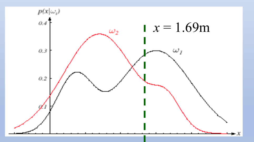
Reading the figure:
- each curve is the class-conditional PDF of height for one class
- at the marked height m the figure compares only the two curves , while the decision compares with , so the priors must still be multiplied in
- each curve is a full distribution over all heights, so it adds up to 1:
For a continuous , is a density. Its height is not a probability and can be larger than 1. Only the area under it over an interval is a probability.
Knowing at every for every class is the big challenge. Later notes meet it by assuming a shape for (the Gaussian) and estimating its few numbers from samples. They also simplify the computation by evaluating one score per class and picking the largest, which turns the decision into classification.
Why do we need this
The posterior is what the MAP rule needs, but the prior and the class-conditional probability are what we can actually measure. Bayes formula joins them, and dropping makes the decision simpler.
Next step
Probability of Error measures how good the MAP rule is over all values of , not just one.
Visual 1: Bayes formula as areas
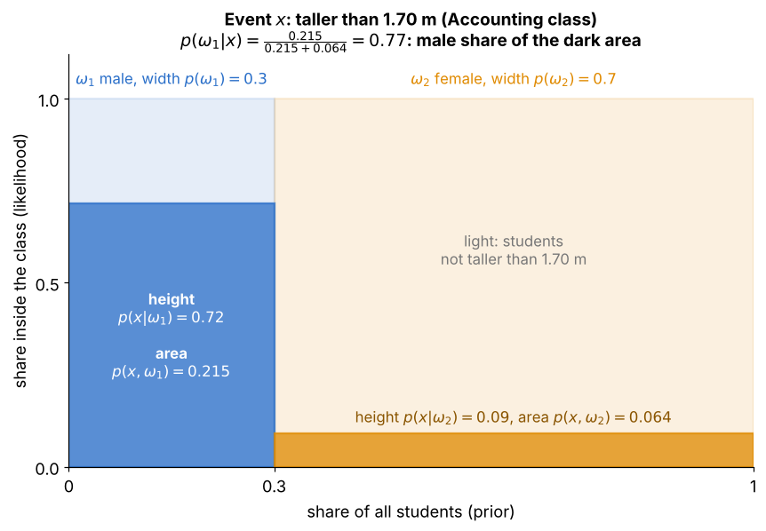
Accounting classroom, with the event "taller than 1.70 m" as :
- the width of each column is the prior , and the dark part of each column has height , the share of that class that is tall
- so each dark area is width times height, the chain rule
- the two dark areas together are , the law of total probability
- the posterior is the male share of the dark area, , even though males are only of the students
Visual 2: mixture as a stack of two curves
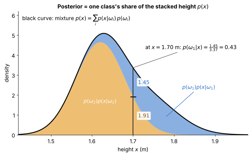
Same classroom, now with height as a density:
- the orange area is , and the blue area sits on top of it as
- the black outline is their sum, the mixture of all students
- at m the stack has height , of which is blue, so
- dividing by only rescales the stack, so comparing the two pieces is enough to decide, as in Step 5
- here is for a height of exactly m, while Visual 1 gave for the event taller than m, so the two do not clash
Visual 3: threshold moves with the prior
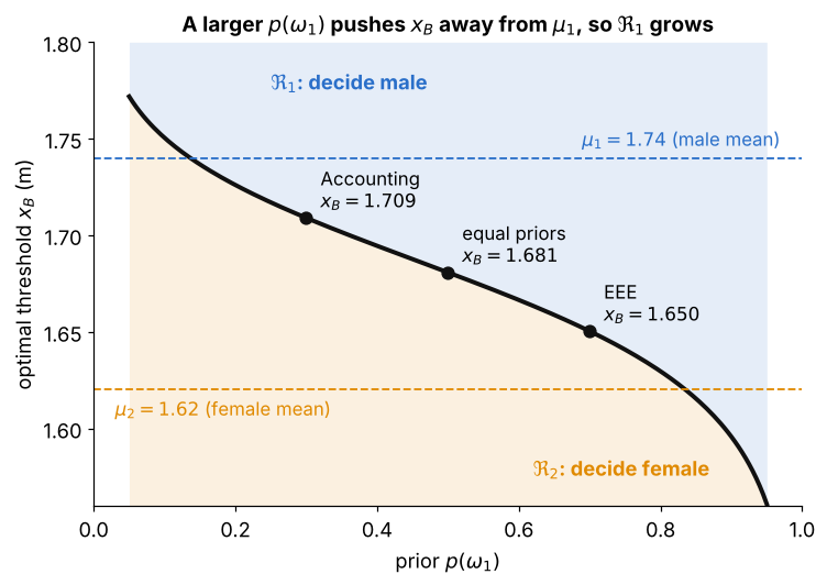
How to read it:
- the black curve is the optimal threshold from , solved for each prior
- as grows, falls away from the male mean , so the region above the curve grows
- Accounting, equal priors and EEE give , and m
- for extreme priors can even pass the other class's mean: a very common class wins most close calls