Hierarchical Clustering (HC)

Hierarchical clustering groups data by building a tree of nested clusters rather than by producing a flat set of groups. The tree is drawn as a dendrogram, where the vertical axis is cluster distance and every join shows 2 groups merging.

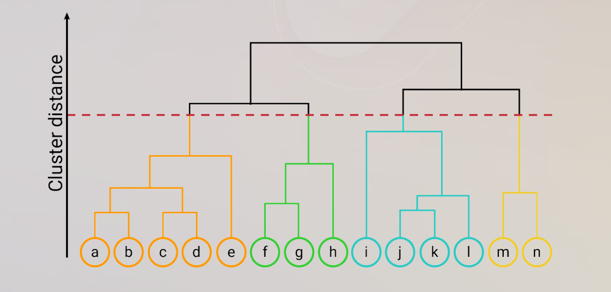
The number of clusters does not need to be fixed in advance. The tree is built once, and then it is cut at a chosen height to obtain the desired number of clusters. A cut low down gives many small clusters, and a cut high up gives a few large ones.

2 Approach to HC

Approach	Starting point	What it does	Direction on the tree
Agglomerative	every object is its own cluster	merges clusters using a distance metric until only 1 cluster remains	bottom up
Divisive	all objects sit in 1 cluster	splits clusters using a distance metric until every object is its own cluster	top down

agglomerative is the version used in practice, since merging is cheaper to compute than searching for the best split
both produce a dendrogram, so the choice affects how the tree is built and not what it looks like

Reading a dendrogram

the leaves at the bottom are the individual data points
each horizontal join marks 2 clusters merging into 1
the height of a join is the distance between the 2 groups at the moment they merged, so a tall join means 2 dissimilar groups were forced together
drawing a horizontal line across the tree and counting the vertical lines it crosses gives the number of clusters at that cut

Example

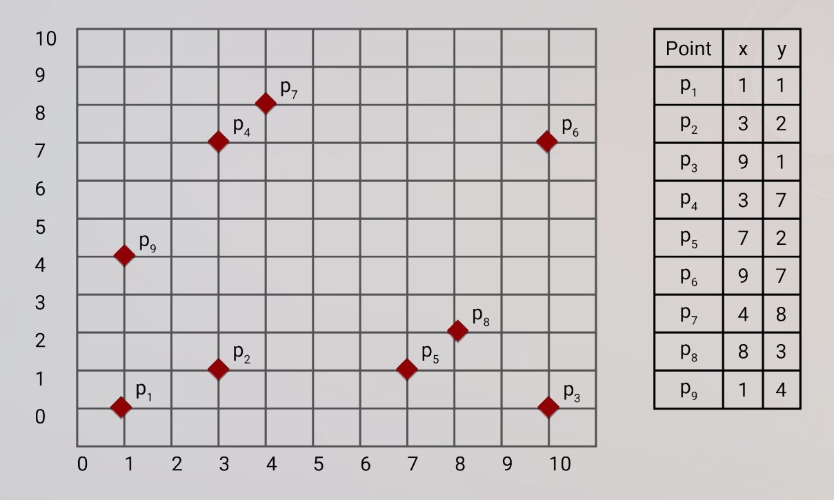
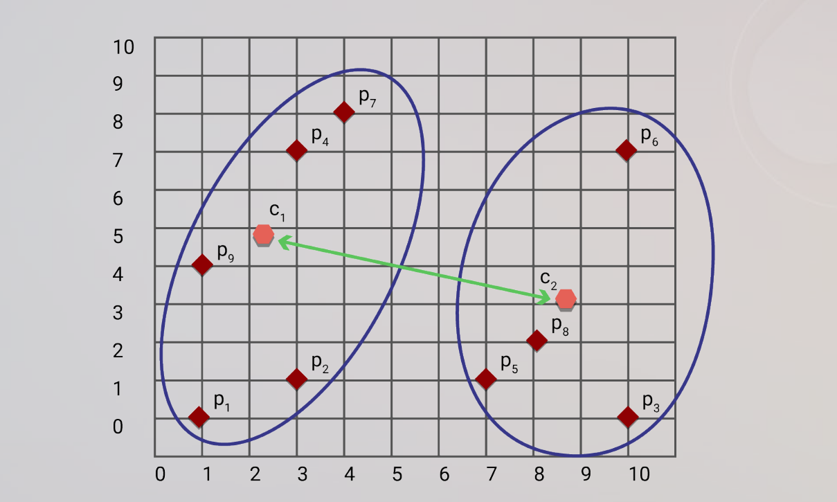
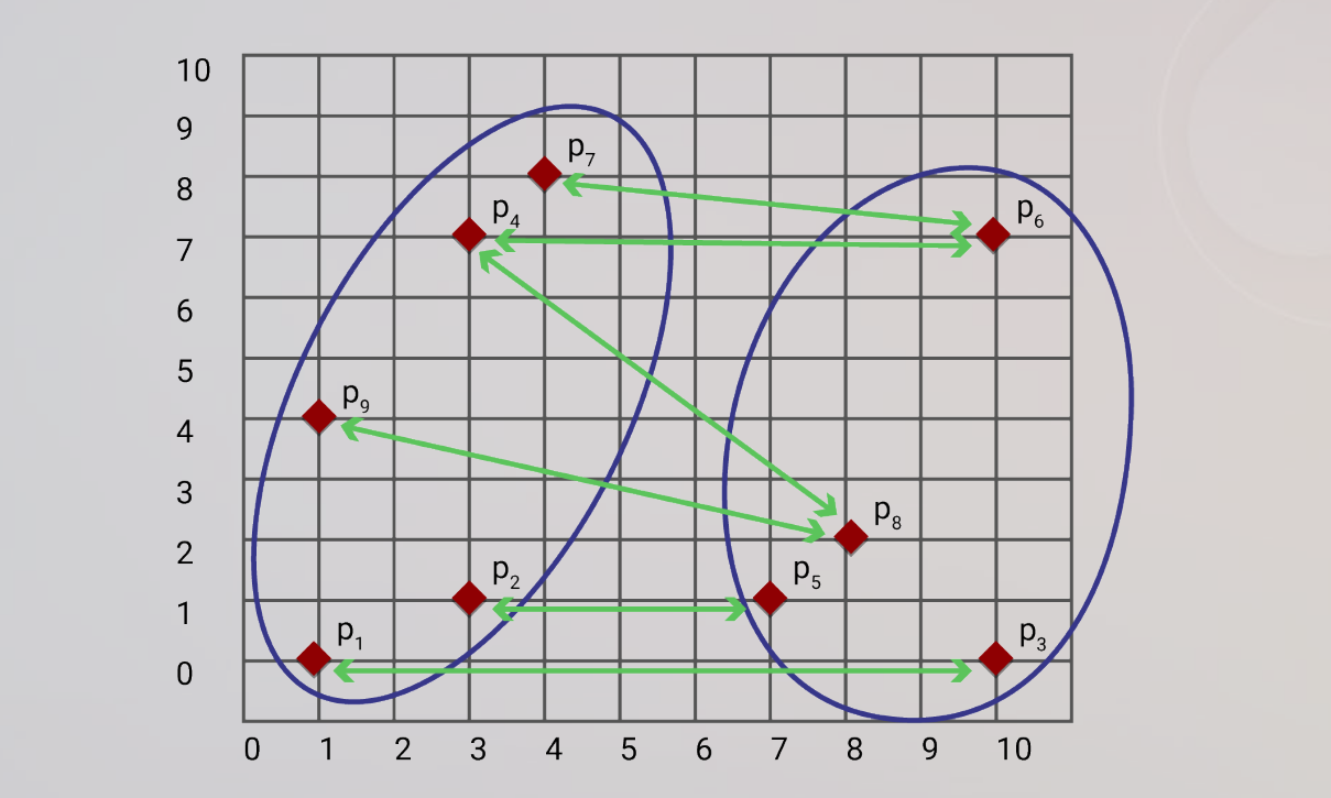
Split into 2 clusters, the groups come out as:

left cluster: $p_{1}$ , $p_{2}$ , $p_{4}$ , $p_{7}$ , $p_{9}$
right cluster: $p_{3}$ , $p_{5}$ , $p_{6}$ , $p_{8}$

The question each linkage method answers is the same. Given these 2 groups of points, what single number should be called the distance between them.

Linkage methods

1. Min Linkage

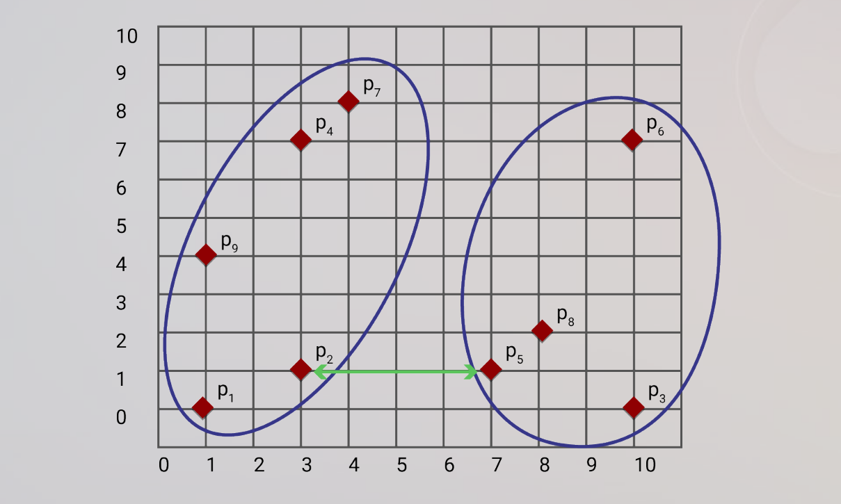
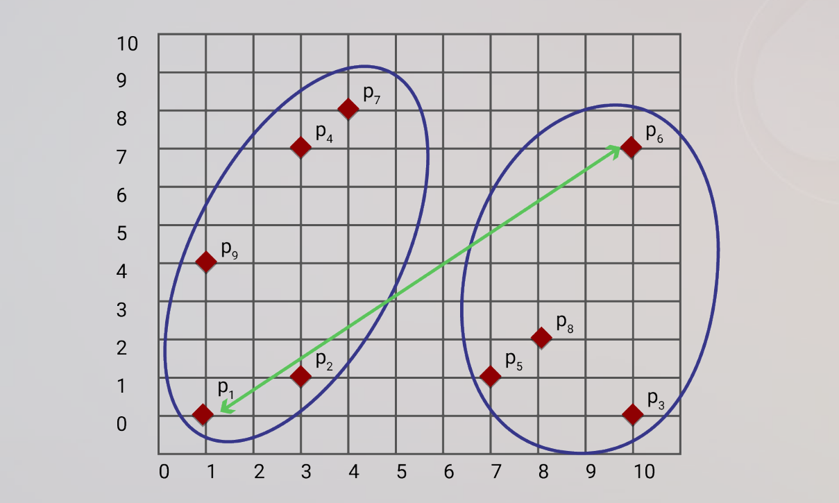
2. Max Linkage

3. Centroid Linkage

4. Average Linkage

Method	Distance between 2 clusters (1 from each cluster)
Min linkage	the distance between the 2 closest points
Max linkage	the distance between the 2 farthest points
Centroid linkage	the distance between the 2 cluster centres
Average linkage	the mean of the distances over every pair of points
Ward linkage	the variance between the clusters, rather than a direct distance between them

min and max both rest on 1 pair of points, which is why a single unusual point can move the answer
average and ward use every point, so they resist outliers better
ward is the method to reach for unless there is a reason to prefer another

Code

These are the 2 libraries that we can use.

from scipy.cluster.hierarchy import linkage, dendrogram, fcluster
import matplotlib.pyplot as plt
 
# Compute linkage matrix, using ward method. Change the method for different linkage
linkage_matrix = linkage(X, method='ward')
 
# Assign clusters
clusters = fcluster(linkage_matrix, t=2, criterion='maxclust')
print("Cluster Assignments:", clusters - 1)
 
# Plot dendrogram
dendrogram(linkage_matrix)
plt.show()

from sklearn.cluster import AgglomerativeClustering
 
hc = AgglomerativeClustering(n_clusters=2, linkage='ward')
labels = hc.fit_predict(X)
print("Cluster Assignments:", labels)

Step	scipy	sklearn
build the tree	`linkage(X, method='ward')`	done inside `fit_predict`
choose the number of clusters	`fcluster(..., t=2, criterion='maxclust')`	`n_clusters=2`
name of the linkage argument	`method`	`linkage`
draw the dendrogram	`dendrogram(linkage_matrix)`	not available directly

method and linkage both accept 'ward', 'single', 'complete', 'average' and 'centroid', where 'single' is min linkage and 'complete' is max linkage
the linkage matrix holds the full merge history, so 1 call to linkage supports any number of clusters afterwards
criterion='maxclust' tells fcluster to read t as a cluster count, and other criteria read t as a distance threshold instead
fcluster numbers clusters from 1, so subtracting 1 lines the labels up with the 0 based labels used elsewhere
the dendrogram needs the linkage matrix rather than the raw data, so it comes from the scipy route

Comparison with K-Means

Point of difference	Hierarchical	K-Means
number of clusters	chosen after the tree is built, by cutting it	fixed before fitting, through `n_clusters`
randomness	none, so the same data gives the same tree every time	centroids start at random positions, so results shift between seeds
output	a full tree of nested groupings	1 flat set of groups
cost	grows quickly with the number of documents, since distances between all pairs are needed	scales better to large corpora

the dendrogram is the reason to choose hierarchical clustering, because it shows structure at every level rather than 1 chosen level
the cost is the reason to choose K-Means on a large corpus

Hierarchical clustering does not need the number of clusters in advance, which is the main thing it does differently from K-Means Clustering.

JJ

Explorer