Point Processing

Motivation

• when we underexpose, overexpose an image
• the gray-level distribution will be a problem

The image above shows the distribution of pixel value with respect to the range of values that a single pixel can have [0-255].

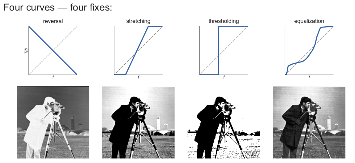
The above image shows 4 different fixes for this issue. These 4 fixes are each their own Transfer Functions, represented as $\mathbf{T}(\mathbf{f})$.

What is Point Processing

• Point processing is where the ouput depends on one pixel only
• in otherwords, a unique pixel undergoes transformation, resulting in a new value for that particular pixel. So we apply point processing on all the unique pixels in an image
• Transfer Function, $T$ in point processing, is represented as a gray-level lookup table
• $T$ is the transformation, or the function that changes the value of our point/pixel

$$g=T(f)$$

where:

• $f$ is the input image captured by the camera
• $g$ is the processed output image
• $T$ is the transformation or operator applied

Gray-level in this case is the level of greyness (0-255) of a particular pixel. A Gray Lookup Table is otherwise known as LUT or lookup table. This lookup table is a literal lookup table like in Python's dictionary or excel's vlookup. In Python, it follows this format:

LUT = {2: 2, 3: 5, 4: 7}

We read this as:

• if any pixel has a value of 2, it stays at 2
• if any pixel has a value of 3, it willl undergo transformation and be changed to 5
• if any pixel has a value of 4, it will undergo transformation and be changed to 7

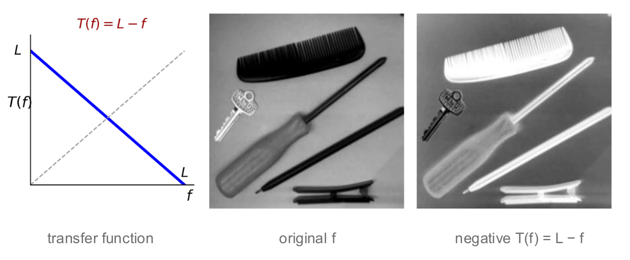
Method 1: Gray-Level Reversal

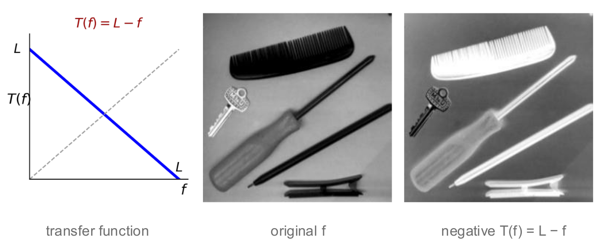
• this is where we convert each pixel from being dark to bright and vice versa

$$T(f)=L-f$$

where:

• $L$ is the maximum possible gray-level value

Method 2: Contrast Stretching

• Problem: flat and grey image, not enough contrast
• Solution: we apply contrast stretching so that the histogram occupies the full gray-level range

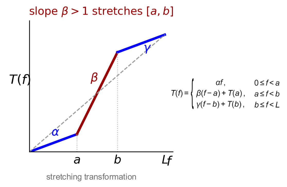
• this method is to set 2 different thresholds, a and b
• a is for the lower limit, while b is for the upper limit
• those pixels with gray-level below a, will be multiplied to a constant $\alpha$
• those pixels with gray-level between a and b, will be multiplied with constant $\beta$
• those pixels with gray-level more than b, will be multiplied with constant $\gamma$

Contrast stretching stretches the signal band [a,b], and ensures the slope $\beta >1$, where the tail is compressed.

Method 3: Clipping

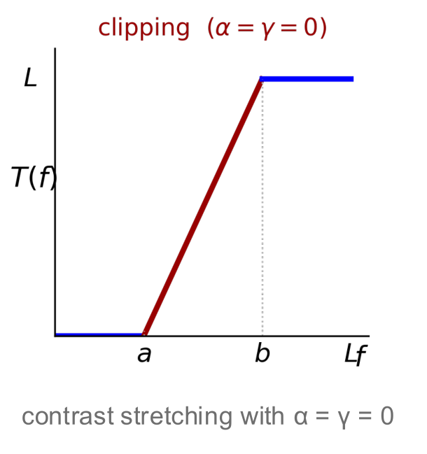
• this is where we only keep [a,b]
• note that $\alpha =\gamma =0$
• it keeps the band with the signal and removes background noise

Method 4: Thresholding

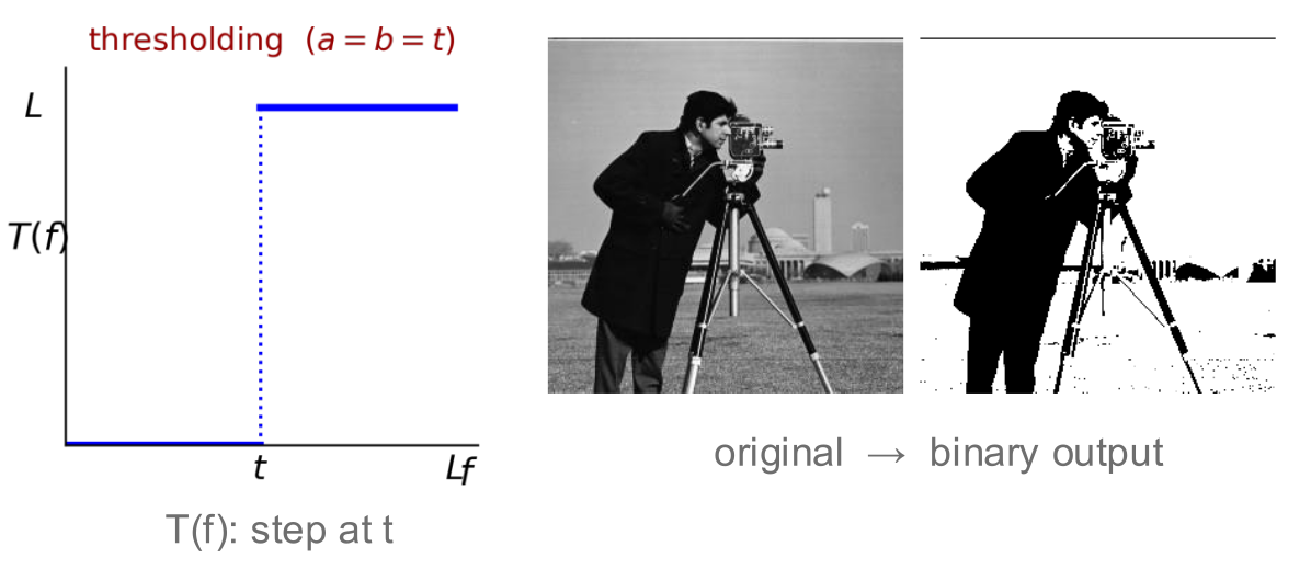
• this is setting a certain threshold, $t$, those pixels above this will be given max possible grey-level, ($L$) and those pixels below this threshold, $t$ will be given a grey-level of $0$
• this binary output is the basis of segmentation

Method 5: Range Compression

Problem:
Some image formats contain a huge variation in values (large dynamic range). For example, the raw calculated values of a Fourier transform spectrum can range from 0 to over 1,000,000.

Screens only has an 8-bit display range, i.e. 256 gray-levels (from 0 to 255). If we try to fit the massive dynamic range into the 256 gray-levels, the single highest peak value will dominate.

Solution:
We can use Logarithmic Transformation.

$$g=clo{g}_{10}(1+f)$$

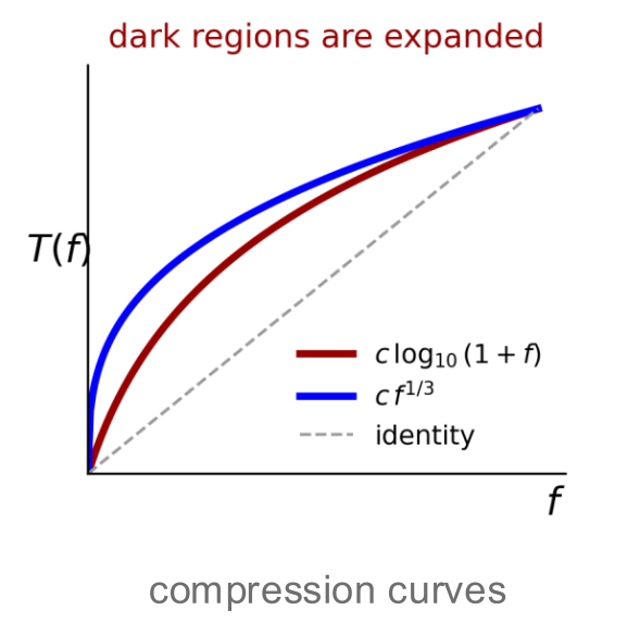
• log helps to make dark values visible
• $c$ is the scaling constant, usually $c=\frac{255}{lo{g}_{10}(1+f_{max})}$ which scales compressed values back into the standard display range of 0 to 255

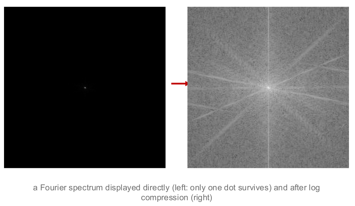
This image shows the results of applying log based scaling.

Histogram

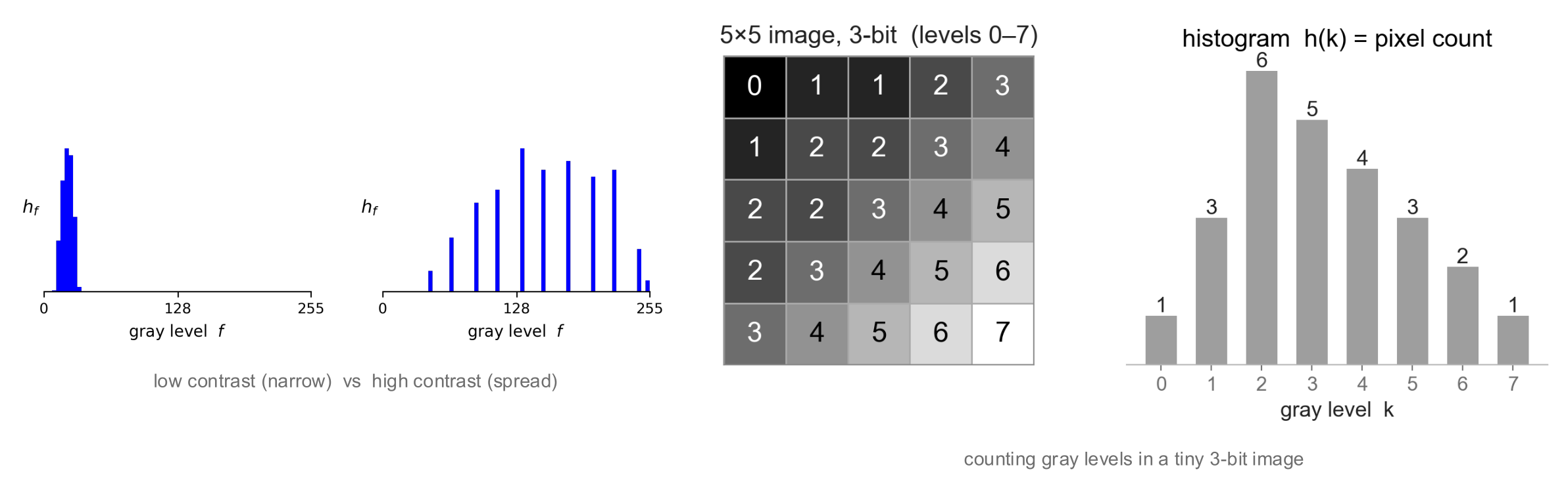
Key components:

• $h(k)=$ pixel count at grey level $k$ (number of pixels with this particular gray level)
• $p(k)=h(k)/MN$ (probability of pixel with grey level $k$, $MN$ are height and width of image)
• a narrower histogram means its lower in contrast

Histogram Equalization

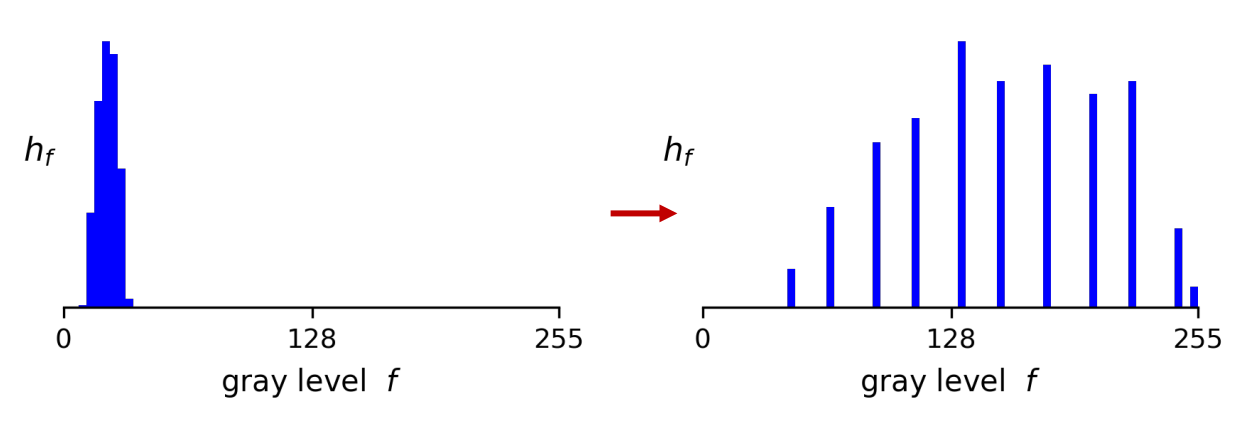
• this purpose is to use all gray levels equally as illustrated above
• the mapping comes from the image itself to no tuning etc

$$c(f)=\sum _{k=0}^{f}p(k),\text{for }f=0,1,\dots ,L$$

where:

• $c(f)$ is the Cumulative Distribution Function (CDF) of the image's grey levels
• it is something like the crowdedness of the histogram's darker and mid-tone bins
• in other words, it is the fraction of pixels that are less than or equals to $f$

$$g=\text{Round}\left[\frac{c(f)-c_{\min }}{1-c_{\min }}(L)\right]$$

where:

• $c_{min}$ is the minimum non-zero cumulative probability value in the image
• $c_{min}$ acts as a stretching offset
• $c_{min}$ here CANNOT be 0, must be minimum non-zero value
• $round$ will round up if its above $.5$ and down if below it

Very Important: L here means the maximum POSSIBLE gray level. Meaning if total we have 8 total number of gray levels, the maximum possible gray level we can have is 7 since we start from 0. This affects how we use the equations above (lecture notes wrote L-1)