Introduction
Discriminant functions need . The most used model for is the multivariate Gaussian, which needs only a mean vector and a covariance matrix per class. This note first builds the mean and covariance, then reads the Gaussian formula, then takes its log to get the score. The score is a quadratic function of , and the Mahalanobis distance appears in it directly. It is the starting point of the quadratic, linear and minimum distance classifiers.
Main idea
For $p(\mathbf{x}|\omega_i)=N(\boldsymbol{\mu}_i,\boldsymbol{\Sigma}_i)$, $g_i(\mathbf{x})=-\frac{1}{2}(\mathbf{x}-\boldsymbol{\mu}_i)^T\boldsymbol{\Sigma}_i^{-1}(\mathbf{x}-\boldsymbol{\mu}_i)+\ln p(\omega_i)-\frac{1}{2}\ln|\boldsymbol{\Sigma}_i|=-\frac{1}{2}d_{\Sigma_i}(\mathbf{x},\boldsymbol{\mu}_i)+b_i$. The class whose mean is closest in Mahalanobis distance wins, with two corrections in $b_i$: one for how common the class is, and one for how spread out it is.
Overview
Sizes, with of components: is , is , and and are single numbers.
Step 1: mean and covariance of a class
The mean of class is the centre of its cloud of points:
The expectation of a vector is taken component by component.
The covariance matrix describes the shape of the cloud:
Why the outer product gives the right entries. For an offset , entry of is , so entry of is :
- a diagonal entry () is the variance , how far feature spreads from its mean
- an off-diagonal entry is the covariance of features and : positive if they tend to be above their means together, negative if one tends to be above when the other is below, and zero if they are uncorrelated
- swapping and gives the same number, so is symmetric,
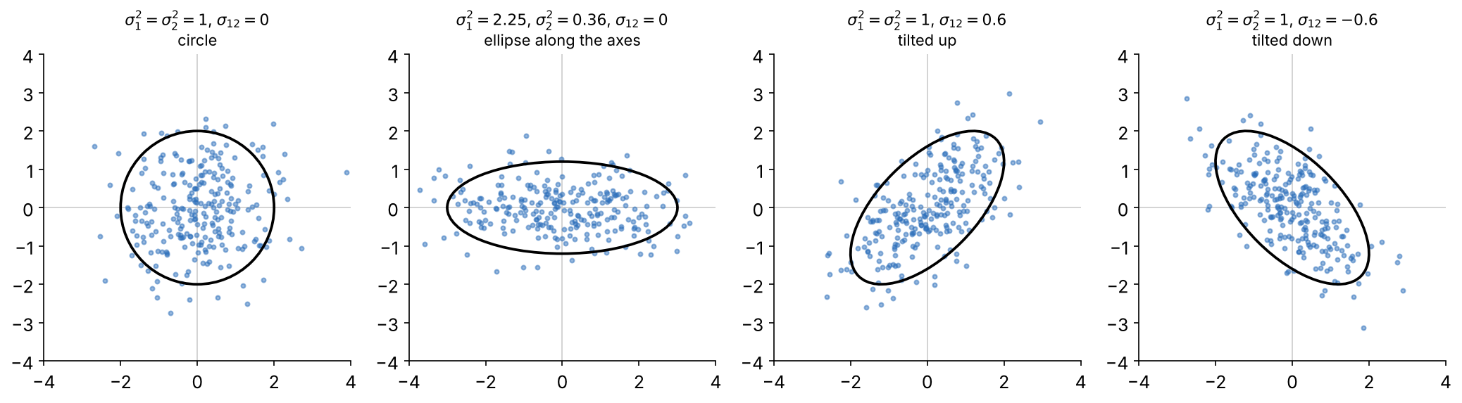
Shape of the cloud, from left to right:
- equal variances and no covariance, , give a circle
- different variances and no covariance give an ellipse along the axes, longer in the feature with the larger variance
- a positive covariance gives an ellipse tilted up, and a negative covariance gives an ellipse tilted down
So the diagonal sets how wide the cloud is along each axis, and the off-diagonal sets how much it tilts.
Estimating from samples. In practice and are unknown. Given samples of the class, replace each expectation by an average:
One element at a time, with as feature of sample :
Three points about the estimate:
- is the maximum likelihood estimate, the value that makes the samples most probable (see Gaussian ML Estimates), and is the unbiased estimate, which is right on average over many sample sets, and they are almost the same for large
- with equal priors, scaling every by the same positive number does not move a linear boundary, so and give the same boundary there
- uses only the offsets , so two classes with the same list of offsets have the same covariance: moving a cloud changes its mean but not its shape
Step 2: multivariate Gaussian
In 1D, with mean and variance :
How to read it:
- is the squared number of standard deviations between and the mean
- turns that into a height that is largest at the mean and drops quickly away from it
- scales the curve so its total area is 1, so a wider curve is lower
In dimensions, the class-conditional PDF is:
Each piece has the same job as in 1D:
| Piece | Meaning | 1D version |
|---|---|---|
| offset of from the centre | ||
| rescales the offset by the spread and tilt of the class: it squashes the class cloud into a round ball (whitening), so the distance becomes an ordinary one | ||
| one number: squared distance in units of spread | ||
| determinant, how much space the cloud covers | ||
| makes the total volume 1 |
With and , the formula becomes the 1D one exactly.
Step 3: take the log
Put the Gaussian into . Two log rules do the work:
- the of a product is the sum of the s, and , so the exponent comes down unchanged
So the discriminant function becomes a quadratic function of :
Step 4: distance plus bias
The term is the same for every class, so it can be dropped. Collect the terms that do not depend on into one number per class:
where:
is the squared Mahalanobis distance from to the class mean, and is a bias that does not depend on .
Step 5: what each term does
| Term | What it measures | Effect on the score |
|---|---|---|
| how far is from the class mean, in units of the class spread | the closer, the higher the score | |
| how common the class is | a common class scores higher | |
| how much space the class covers | at the same Mahalanobis distance, a tight class scores higher than a spread-out one |
Why the spread term is there:
- a spread-out class shares its probability over a large volume, so its density is lower everywhere
- a tight class packs its probability into a small volume, so its density near its mean is high
- is how this shows up in the score
So the score reads: how well does fit class , adjusted for how common the class is.
Step 6: three cases
What happens next depends only on the covariance matrices of the classes. This table is a preview: the quadratic term appears when the distance is multiplied out, which Quadratic Classifier does. A hyperplane is the set where a linear equation in is zero (a line in 2D, a plane in 3D), and a hyperquadric is the set where a quadratic equation is zero (a curve such as an ellipse or a hyperbola in 2D).
| Covariance | What cancels in | Boundary | Classifier |
|---|---|---|---|
| different | only constants | curved (hyperquadric) | quadratic |
| one shared | the term and | hyperplane | linear |
| shared | the same, and only rescales | hyperplane perpendicular to the line of means | minimum distance (with equal priors) |
All three are the same Bayes classifier. Each step down the table adds a stronger assumption and gives a simpler formula, and each is only optimal when its assumption is true.
Why do we need this
It turns the general Bayes rule into a formula you can evaluate with a mean, a covariance and a prior, and these can be estimated from samples. It also shows the idea that ties all Gaussian classifiers together: pick the nearest class mean, with distance measured the right way.
Next step
Mahalanobis and Euclidean Distance explains the distance inside the score.
Visual 1: three terms of the score at one point
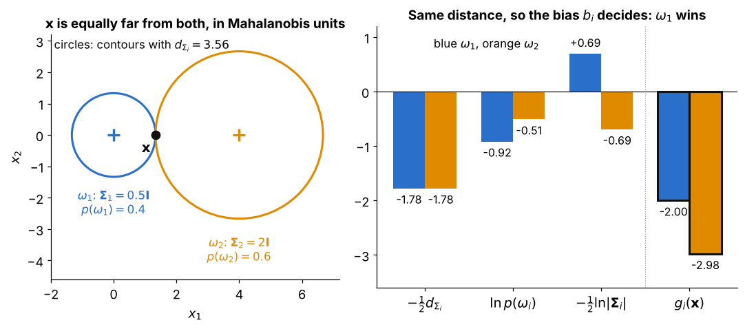
A tight class and a spread-out class :
- left: lies on a solid contour of both classes, so it has the same Mahalanobis distance to both means
- right: the distance terms are equal, favours the more common , and favours the tight
- the spread term wins here, so beats and goes to
- this is the score of Step 4, , with the bias split into its two parts
Visual 2: covariance from products of offsets
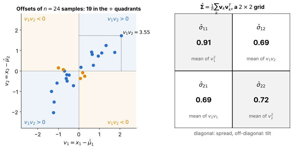
How to read it:
- each dot is the offset of one sample, so the cloud is centred on zero
- in the blue quadrants , and in the orange ones ; here of points are blue
- is the average of , so the blue majority gives a positive and an upward tilt
- the diagonal entries average and , which are never negative, so they only measure spread