Swin Transformer

Important Terminologies to Understand:

(1) $A\times B$ grid of windows refers to $AB$ total number of windows

• when we say a $A\times B$ grid we mean the number of windows wrt both height and width
• A refers to the number of windows wrt the full height of the image
• B refers to the number of windows wrt the full width of the image
• grid usually means a literal grid of windows, similar to how we split an image up into 4 patches, we have a $2\times 2$ grid of images

(2) Image divided into $A\times B$ patches

• the $A\times B$ here refer to the actual size per patch
• meaning from an image of $224\times 224$, we will get $\frac{224}{A}$ number of patches wrt the width, and $\frac{224}{B}$ number of patches wrt the height
• resulting in a total of $\frac{224}{A}\times \frac{224}{B}$ number of patches

Part 1: Hierachical Feature Maps

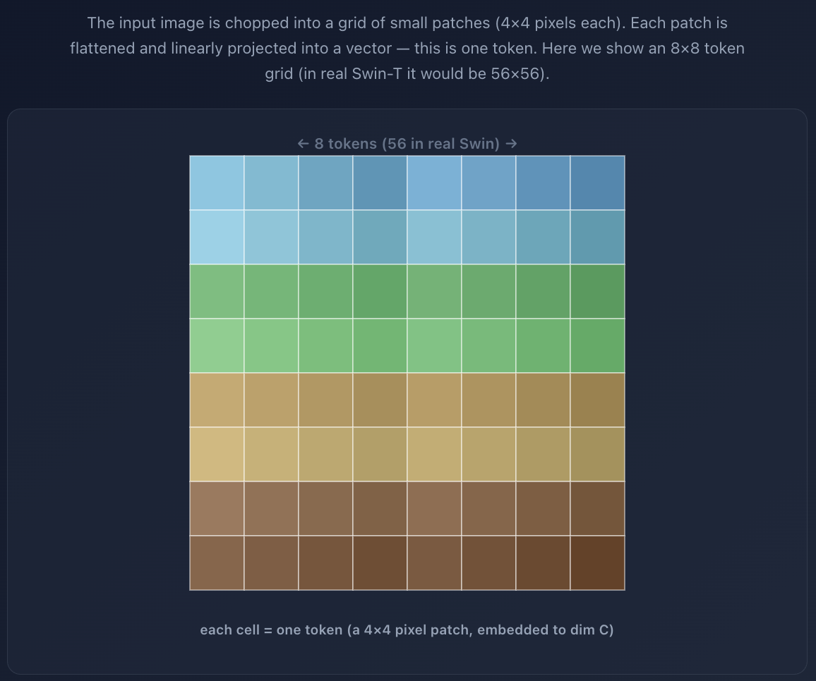
• in ViT, images split into patches
• these patches remain the same size throughout every single layer of the network
• this produces a single-resolution feature map which is bad for dense predictions like detecting small objects
• swin transformers fixes this my mimicking the structure of traditional CNNs
• it build a hierachical feature map by merging patches as the network gets deeper

Input

• We start with an image of size $H\times W\times 3$ (Height, Width, Channels - RGB)

Stage 1

• Images divided into small patches (usually $4\times 4$ pixels)
• This gives a feature map resolution of $\frac{H}{4}\times \frac{W}{4}$

Stage 2, 3 and 4

• As tokens move deeper into the network, neighbouring patches are systematically merged together (e.g. $2\times 2$ neighbouring patches become 1 token)

Final

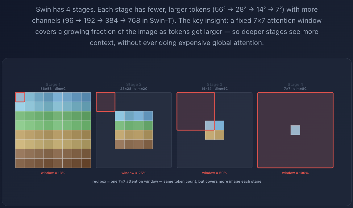
• By the final stage, spatial resolution drops to $\frac{H}{32}\times \frac{W}{32}$
• just like CNN, swin transformer's feature map starts large with great details
• we say 'large' because with a $4\times 4$ patches in a $224\times 224$ image, we will end up with a large grid of $56\times 56$ individual results
• many $4\times 4$ pixels patches will show us great small level details such as corners, textures, sharp edges
• moving up to stage 4, we will end up with a high-level overview of the image with larger patches
• these large patches are able to look at features such as shape and whole objects

Part 2: Linear Embedding and Patch Merging

Stage 1: Patch Partition & Linear Embedding

• the $4\times 4$ patches (of $4\times 4\times 3=48$ values) are flattened
• resulting in $48$ raw pixel values in a vector form
• we pass this through a Linear Layer to a specified channel dimension, denoted as $C$ (an arbitrary hidden size, like 96)
• meaning each patch will now be a single 1D vector of length C
• this transforms our $\frac{H}{4}\times \frac{W}{4}\times 48$ raw pixel grid into a clean token grid of shape:

$$\frac{H}{4}\times \frac{W}{4}\times C$$

Stages 2, 3, 4: Patch Merging

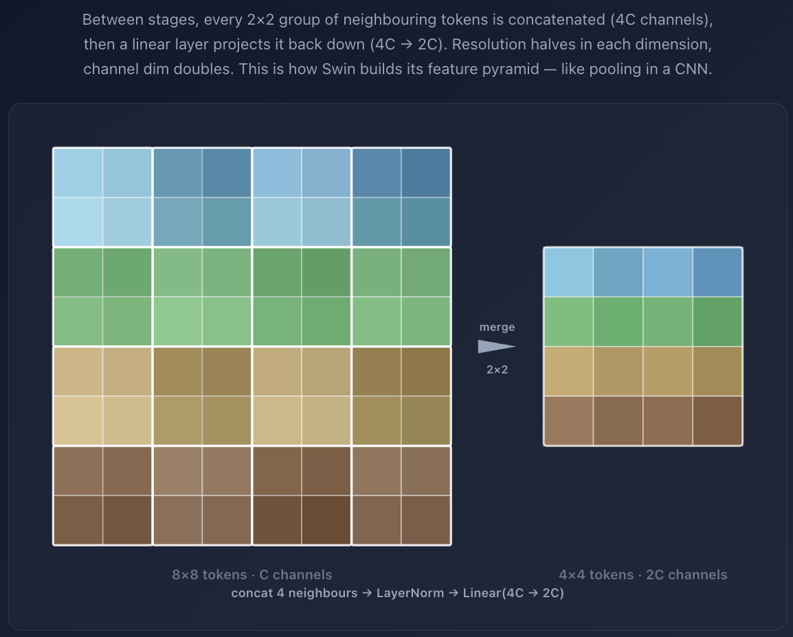
• to downsample the spatial grid and increase the channel depth as we move deeper, the network uses a Patch Merging layer
• it acts like a pooling layer in CNN, but it doesn't throw away any data

Between Stage 1 and Stage 2:

(1) Concatenate

• it takes groups of $2\times 2$ neighbouring patches and concatenates their features together
• gluing 4 neighbours together gives a single token with $4C$ channels

(2) Downsample

• since we group $2\times 2$ patches into 1, the spatial grid resolution is cut into half (reduced)
• from $\frac{H}{4}\times \frac{W}{4}$ down to $\frac{H}{8}\times \frac{W}{8}$

(3) Linear Reduction

• To keep channel count from blowing up too fast, a linear layer projects the $4C$ down to $2C$
• meaning that initially our 4 combined patch has a combined length of 4C, but then because we linearly project it onto a linear layer, we reduce the length of vector to $2C$

(4) Pattern

• this pattern continues between stages
• every time you pass through a Patch Merging layer, the spatial resolution is halved, and the channel depth is doubled.
  • Stage 1: $\frac{H}{4}\times \frac{W}{4}\times C$
  • Stage 2: $\frac{H}{8}\times \frac{W}{8}\times 2C$
  • Stage 3: $\frac{H}{16}\times \frac{W}{16}\times 4C$
  • Stage 4: $\frac{H}{32}\times \frac{W}{32}\times 8C$

Note: $C$ refers to the Stage 1 output dimension, not the raw pixel vector length

Part 3: Window-based Self Attention

• Swin introduces Window-based Self-Attention
• this W-MSA runs inside every stage

How W-MSA works:

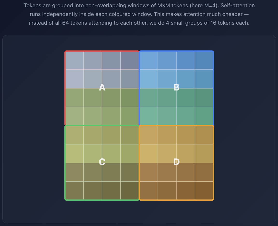
• swin divides the feature map into a grid of non-overlapping windows
• the original paper uses a standard window size of $7\times 7$
• self-attention is only calculated within each individual window
• a patch is window A can only talk to other patches in window A

Math:

• since attention is confined to a fixed $7\times 7=49$ tokens
• the cost to calculate attention inside a single window is always constant $(49^2)$
• if we scale up the image size, we can just add more windows
• this changes the computational cost from quadratic $O(N^2)$ to linear $O(N)$

Part 4: Shifted Window Attention

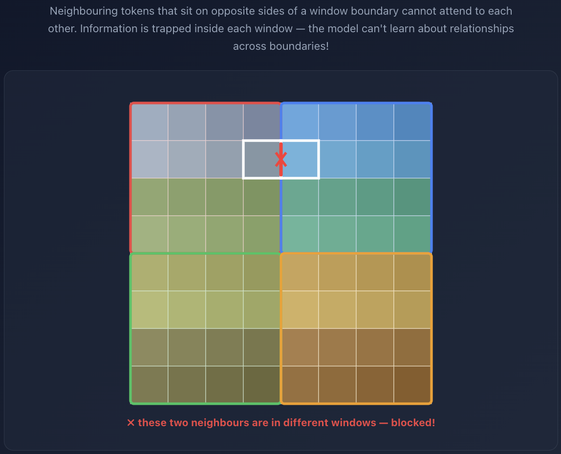
• windows are isolated
• swin transformers come in a pair of 2 consecutive blocks:
  • Block 1 uses Regular Windowing (W-MSA) which is explained in Part 3
  • Block 2 uses Shifted Windowing (SW-MSA)

How SW-MSA works:

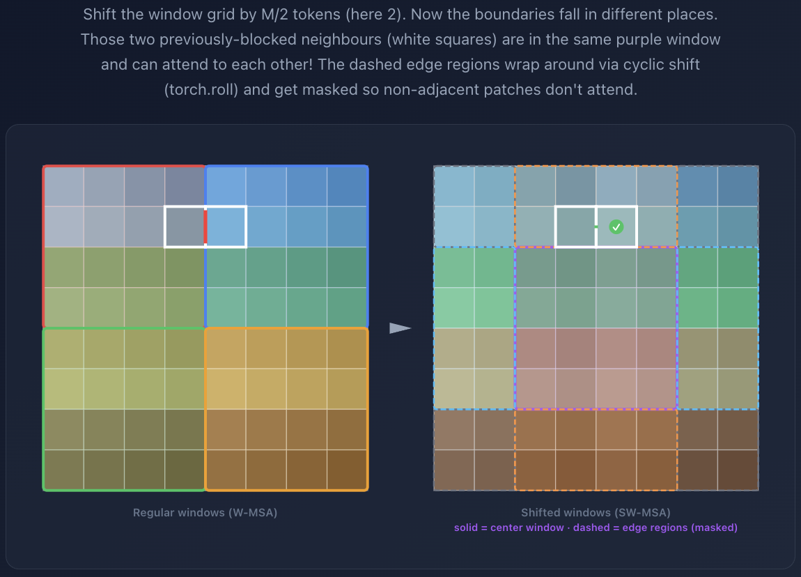
• SW-MSA starts from the same partition as W-MSA (many $7\times 7$ windows)
• when we shift, we slide the entire window grid down by $\lfloor \frac{M}{2}\rfloor$ pixels, i.e. shift amount is the floor of $\frac{M}{2}$
• the paper used a window size of $7\times 7$, which means we shift the grid by 3 patches down and 3 patches right
• By shifting the boundaries, the new windows are centered directly on top of the old boundaries.
• Patches that were once seperated into 2 different windows are now both inside the same window because of this shifting mechanism
• They can now run self-attention together, passing information across the old borders

Part 5: Cyclic Shifting & Masking Attention

Step 1: Cyclic Shifting (Realignment)

• when we shift windows down and right, the parts left over at the top and left edges are phyiscally moved to the opposite side
• so what we do is shift these orphaned patches around the edges to join other orphaned patches, forming a complete 7x7 window
• something like pac-man wrapping effect
• so the left orphan flies off the left edge to join the right orphan at the right side
• top orphan flies off the top and comes out at the bottom to join the bottom orphan
• same for the corner orphan flying off and joining diagonal orphan at the opposite corner

Step 2: Masked Attention (The Correction)

• since these "edge cases" sub-sections within those windows are spatially non-adjacent to other sections
• we apply something called Masked Attention onto these "edge cases"
• During the attention calculation ($Q\cdot K^T$), the model applies a matrix mask
• masks sets those "edge cases" windows' attention scores to $-\infty$, effectively blocking them from communicating
• note that it only applies this mask on unrelated groups to $-\infty$
• for example, if a window contains 2 patches physically side by side, and 2 patches totally unrelated, mask will apply to the 2 unrelated ones only

Step 3: Shift Back

• Once the attention calculation is done inside the shifted window block, the tokens are cyclically shifted back to their original positions to keep the image structure intact for the next layers