Motion Planning and Trajectory

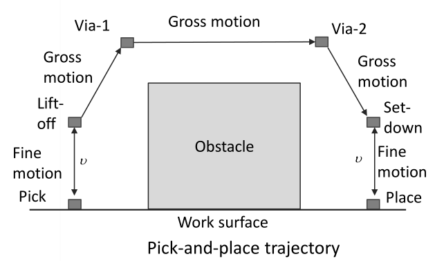
Pick and Place Operation

For simple point to point motion, we can execute pick and place operations using 4 discrete points:

1. pick point
2. lift-off point
3. place point
4. set-down point

1. Pick Point

$$T_{base}^{pick}=\left[\begin{array}{cc}{R}_{pick}& p_{pick}\\ 000& 1\end{array}\right]$$

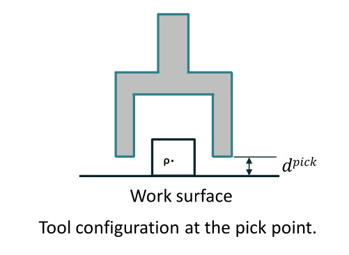
• the coordinate frame is represented above
• this represents the initial position and orientation of the part being manipulated

2. Lift-off Point

$$T_{base}^{lift}=\left[\begin{array}{cc}{R}_{pick}& p_{pick}-v{R}_{pick}{i}^3\\ 000& 1\end{array}\right]$$

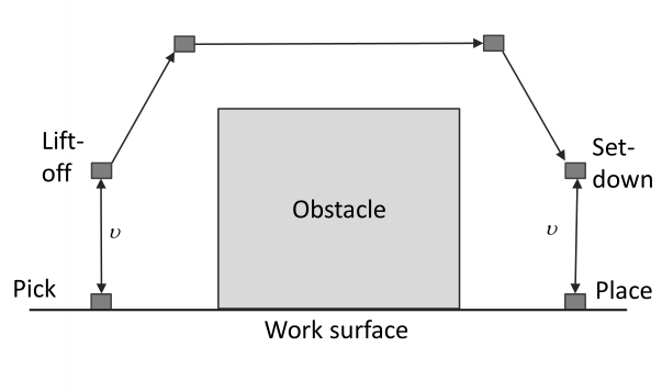
• $v$ is referred to as the approach distance
• TCP orientation at the lift-off point is identical at the pick point

3. Place Point

• Place point is represented as $T_{base}^{place}$
• this is the final position and orientation of the part being manipulated
• the place orientation $R_{place}$ should be selected in such a manner that the approach vector $r^3$ is orthogonal to the surface that the part will come to rest

$$d_{place}=d_{pick}$$

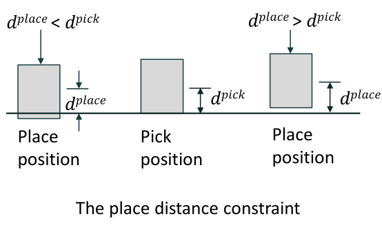
• the distance $d_{place}$ between the place position and the place surface, should be the same as the distance $d_{pick}$ between the pick position and pick surface

When the part is picked up from and placed down into the same common horizontal work surface, we can model the equation as such:

$$p_3^{place}=p_3^{pick}$$

More generally, if parts are being stacked vertically and the vertical seperation between the pick surface and the plane surface is the height of the stack, denoted $h_{stack}$, then the following constraint must be satisfied for a proper stacking operation:

$$p_3^{place}=h_{stack}+p_3^{pick}$$ $$h_{stack}=h_{stack}+2p_3^{pick}$$

4. Set-down Point

$$T_{base}^{set}=\left[\begin{array}{cc}{R}_{place}& p_{place}-v{R}_{place}{i}^3\\ 000& 1\end{array}\right]$$

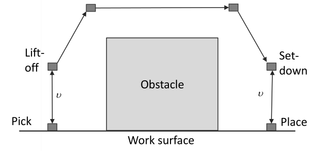
• this is the last point
• it works the same way as the lift-off point
• once the place-point frame has been determined, that associated set-down point frame can be computed

Speed Variations

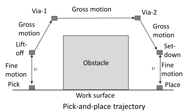
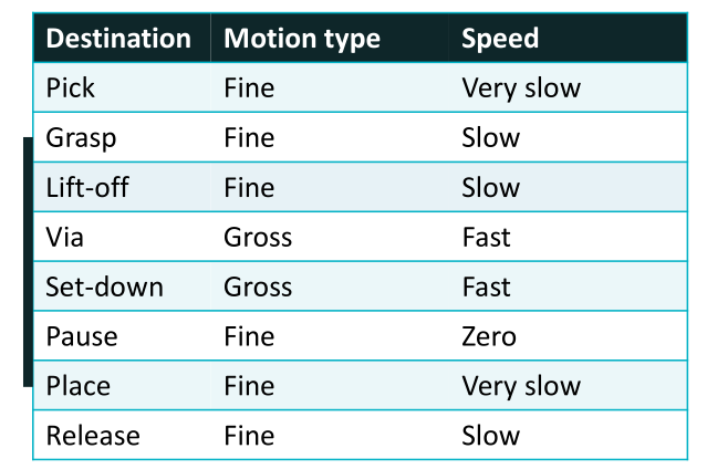
Paths and Trajectories

Continuous-path is crucial for applications where a specifc path must be followed in the workspace. The speed in these scenarios must also be regulated.

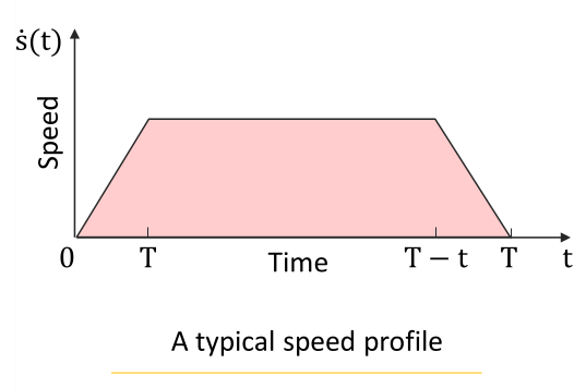
For this continuous path problem, we will use the formulation in tool configuration space $R^6$, represented by:

$$w^1(q)=p(q)$$ $$w^2(q)=\exp \left(\frac{q_n}{\pi }\right)r^3(q)$$

Here is how we can model the continuous-path tool trajectory:

$$\Gamma =\{w(\lambda )\in R^6:0\le \lambda \le 1\},0\le t\le T$$ $$\lambda =s(t)$$

• $\Gamma$ is a curve in tool-configuration space $R^6$, which is the path that the tool is supposed to follow
• $\lambda$ is the normalized path length parameter where $\lambda =0$ represents the start of the path and $\lambda =1$ represents the end
• $s(t)$ is a differentiable speed distribution function mapping $[0,T]$ into $[0,1]$, with $s(0)=0$ and $s(T)=1$
• it tells us which part of the path it is at, so its not the speed function

$$s(t)=\frac{t}{T},0\le t\le T$$

• the equation above is to represent a constant tool speed of $1/T$

Time Derivative of Speed Distribution Function

The time derivative of speed distribution function, $s(t)$, represents the instantaneous speed of the tool tip at time $t$. This is represented as $\dot{s}(t)$.

Our goal is to be able to determine the joint rates that will generate our desired tool trajectory. The $k^{th}$ joint velocity is directly proportional to the output speed of the $k^{th}$ motor or actuator for $1\le k\le n$.

Cubic Polynomial Interpolation

We require knot points and via-points (waypoints) because real path is usually not specific. For the general interpolation problem, there is a sequence of $m$ knot points in the tool-configuration space that must be visited by the tool:

$$\Gamma =\{w_0,...,w_{m-1}\}$$

The path $w(t)$ between the $m$ knot points must be smooth. This requires at least 2 derivatives in order to avoid infinite acceleration.

Simplest case is $m=2$. We have $\{w_0,w_1\}$. Our cubic polynomial path is:

$$w(t)=a{t}^3+b{t}^2+ct+d,0\le t\le T$$

The polynomial coefficients $\{a,b,c,d\}$ are vectors in $R^6$. The 2 position contraints are at the end points of the trajectory:

$$w(0)=w^0,w(T)=w^1$$

These 2 constraints remove 2 of the 4 dof available for choosing the coefficients. The remaining 2 dof can be used to specify the velocities at the end points of the trajectory.

Suppose the robot is to move from point $w_0$ to $w_1$ in tool-configuration space over an interval of time $[0,T]$. If the starting time is 0 and then ending time is $T$ with velocity $v_1$, then:

$$a=\frac{T(v^1+v^o)-2(w^1-w^o)}{T^3}$$ $$b=\frac{3(w^1-w^o)-T(v^1+2v^o)}{T^2}$$ $$c=v^0$$ $$d=w^0$$

Interpolated Motion with parabolic bends

Piecewise-linear interpolation between knot points is efficient but not smooth. The velocity changes abruptly at a knot point, which demands infinite instantaneous acceleration. A parabolic blend replaces the corner with a constant-acceleration arc, so the acceleration stays finite.

Problem Statement

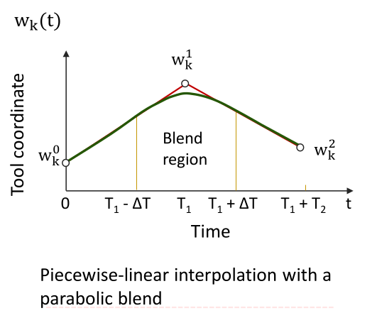
• three knot points $\{w^0,w^1,w^2\}$ in tool-configuration space
• segment traversal times $T_1$ and $T_2$
• blend transition time $\Delta T$, chosen by the user

The blend is centred on the middle knot $w^1$ and runs over the interval $[T_1-\Delta T,T_1+\Delta T]$.

Step 1: Segment Displacements and Velocities

$$\Delta w^j=w^j-w^{j-1},v^j=\frac{\Delta w^j}{T_j},1\le j\le 2$$

Each straight segment is traversed at its own constant velocity.

Step 2: Check the Transition Time

$$0<\Delta T<\min \{T_1,T_2\}$$

Step 3: Blend Acceleration

$$a=\frac{T_1\Delta w^2-T_2\Delta w^1}{2T_1{T}_2\Delta T}$$ $$b=\frac{w^1-w^0}{T_1}$$

$a$ is the constant acceleration that carries the tool from velocity $v^1$ at time $T_1-\Delta T$ to velocity $v^2$ at time $T_1+\Delta T$. Note that $b$ is just the velocity of the first segment.

Step 4: Complete Trajectory

$$w(t)=\{\begin{array}{ll}{w}^0+\frac{t(w^1-w^0)}{T_1}& 0\le t\le T_1-\Delta T\\ \frac{a}{2}(t-T_1+\Delta T{)}^2+\frac{(w^1-w^0)(t-T_1)}{T_1}+w^1& T_1-\Delta T<t<T_1+\Delta T\\ w^1+\frac{(w^2-w^1)(t-T_1)}{T_2}& T_1+\Delta T\le t\le T_1+T_2\end{array}$$

Notes

• the blend is a quadratic in $t$, of the general form

$$w(t)=\frac{a(t-T_1+\Delta T{)}^2}{2}+b(t-T_1+\Delta T)+c$$

• the constant $c$ comes from the position constraint at the start of the transition:

$$w(T_1-\Delta T)=w^1-\left(\frac{\Delta T}{T_1}\right)(w^1-w^0)$$

• the tool does not pass through $w^1$ itself. It cuts the corner inside the blend region

Straight-Line Motion

A straight line is the shortest path between two points, so straight-line trajectories in the workspace are common.

The ideal straight line

Given the initial and final points $w^0$ and $w^1$ in tool-configuration space $R^6$:

$$w(t)=\left(1-s(t)\right)w^0+s(t)w^1,0\le t\le T$$

• $s(t)$ is a differentiable speed distribution function mapping $[0,T]$ into $[0,1]$ with $s(T)=1$
• it either has a ramp-up, constant-speed, ramp-down profile, or the simple form $s(t)=t/T$

Two practical limitations

• if $n<6$, the tool tip cannot follow an arbitrary straight-line path in $R^6$. Most robots can still follow a straight line along the approach vector
• many robots only have point-to-point motion control, so the straight line must be approximated

The approximation is done by visiting a sequence of closely spaced knot points in joint space.

Algorithm 4-8-1: Bounded Deviation

Recursively insert knot points until the joint-space path stays within a tolerance of the true straight line.

1. Select $\epsilon >0$. Use inverse kinematics to compute $\{q^0,q^1\}$, the joint vectors associated with $\{w^0,w^1\}$
2. Compute the joint-space midpoint

$$q^m=\frac{q^0+q^1}{2}$$

3. Use $q^m$ and $w$ to compute the associated tool-configuration space midpoint

$$w^m=w(q^m)$$

4. Compute the exact tool-configuration space midpoint

$$w^M=\frac{w^0+w^1}{2}$$

5. If the deviation $\Vert w^m-w^M\Vert \le \epsilon$, then stop. Otherwise insert $w^M$ as a knot point between $w^0$ and $w^1$
6. Apply the algorithm recursively to the two new segments $\{w^0,w^M\}$ and $\{w^M,w^1\}$

The key idea is that $q^m$ is the midpoint in joint space, while $w^M$ is the midpoint in tool-configuration space. They do not coincide, because the forward kinematics is non-linear. The gap between them is the deviation from the straight line.

This algorithm does not necessarily distribute the knot points uniformly over the interval