Aim
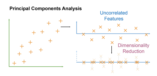
PCA is a linear technique that finds orthogonal axes in the data that capture the most variance.
PCA is very similar to Support Vector Machine, we have the same hyperplane concept, and also trying to maximize distance between points and the hyperplane.
Introduction
- PCA aims to project the data onto a lower-dimensional space while minimising information loss
- PCA works by transforming the original data to a new set of variables called the principal components (PCs)
- the PCs are uncorrelated and can be ordered so that the first few PCs retain most of the variation present in all the original variables of the dataset
How it works
- PCA aims to construct lines (2D), planes (3D) or hyperplanes (>3D) which are unit vectors orthogonal to the original features
- to do this, we minimise the mean perpendicular distance from the PC line for all points:
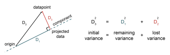
- the function reaches a minimum when = the eigenvector of the covariance matrix of
The variance decomposition behind it:
| Term | Meaning |
|---|---|
| initial variance, which is the distance from the origin to the datapoint | |
| remaining variance, which is the projection onto the component | |
| lost variance, which is the perpendicular distance to the component |
- the goal is to maximise and minimise while keeping constant
Algorithm
Main Idea
PCA can be done manually using the following steps.
- Standardise the data
- Compute the covariance matrix of the dataset
- Derive the corresponding eigenvalues and eigenvectors on the normalised dataset
- PCs can be calculated using the dot product of the eigenvectors and the standardised columns
PCA in Scikit-Learn
Using the same twitter dataset.
1. Apply TF-IDF
from nltk.corpus import stopwords
import nltk
nltk.download('stopwords')
from nltk.corpus import stopwords

stop_words = stopwords.words('english')
stop_words.extend(['https', 'tco'])

vect = TfidfVectorizer(stop_words=stop_words)
X = vect.fit_transform(tweets.OriginalTweet)
tf_idf_vect = pd.DataFrame(X.toarray().transpose(), index=vect.get_feature_names_out())
Output:
1078 rows x 100 columns
- in this DataFrame, each column represents a tweet
- even with stop words removed, the raw TF-IDF vector still has 1078 dimensions
2. Apply PCA to reduce to 50 components
from sklearn.decomposition import PCA

pca = PCA(n_components=50)
pca.fit_transform(tf_idf_vect)
Output:
array([[-1.56131468e-02, -7.07384109e-03, -3.80598744e-02, ...,
        -4.65646897e-02,  1.90040344e-02,  3.94027865e-03],
       [-3.33563752e-02, -3.05233715e-03,  1.21276381e-02, ...,
        -1.65352581e-02,  3.68304283e-02,  4.36982156e-02],
       ...
       [-1.73831820e-02, -1.16869004e-03, -1.42062209e-02, ...,
        -1.35501994e-03, -2.56078477e-02, -3.06579365e-02]])
3. Inspect the components and the variance captured
print(pca.components_)
print(sum(pca.explained_variance_ratio_))
Output:
0.5935386745713639
- the
.components_attribute stores the directions of maximum variance, which are the principal components - with 50 components, almost 60 percent of the variance in the data was captured
Advantages and Limitations
| Advantages | Limitations |
|---|---|
| Visualisation: PCA is valuable for visualising high-dimensional data, since it projects data onto lower-dimensional spaces, which makes it easier to plot and analyse in 2D or 3D | Lack of interpretability: while PCA simplifies data representation, the new features are linear combinations of the original features and may not have clear semantic meaning |
| Feature engineering: PCA can be used for feature engineering by creating new features as linear combinations of the original features, and these new features may have improved discriminative power | Linearity assumption: PCA assumes that relationships between variables are linear, so if the data contains non-linear relationships, PCA may not capture them effectively |
PCA centres the data, so it cannot take a sparse matrix, and the version used on sparse text matrices is Singular Value Decomposition (SVD).